The Transformer Replaced Recurrence With Direct Attention Between Tokens
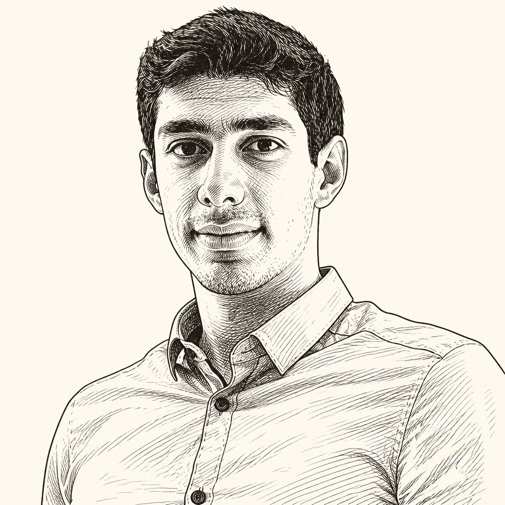
In the opening lecture of Stanford’s CME295 course on transformers and large language models, adjunct professors Afshine and Shervine Amidi explain how the Transformer offered an alternative to recurrent models. They argue that its use of attention let tokens connect directly across a sequence, rather than relying on a recurrent state to carry information forward one step at a time, and helped put language modelling on a more scalable path.

The Transformer changed both what language models could do and how they could scale
Before large language models became general-purpose tools, natural-language systems were usually built for individual tasks. In the 2010s, ? afshine-amidi said, a sentiment classifier, a translation system and a named-entity recognizer would typically be separate models. Recurrent neural networks (RNNs) were prominent: they processed text as a sequence, carrying information from one step to the next.
The change that set the field on a different path came with the 2017 paper Attention Is All You Need. Its Transformer architecture dispensed with recurrence and instead used attention to let tokens connect directly to one another. Amidi described the result as scalable: increasing data, compute and model size could produce larger performance gains than earlier approaches. Researchers subsequently scaled Transformers in both the number of model parameters and the number of training tokens, producing systems that could generate text and code well.
The next shift was in how people used those systems. Shervine Amidi pointed to ChatGPT’s release in 2022 as a product turning point: it introduced many people to interacting with a model through a conversational interface. The instructors placed coding agents in a further, “agentic” phase, where models are used to carry out tasks rather than only answer prompts. The course would return to agents and practical applications later; the first lecture focused on the architecture beneath them.
The lecture’s route to that architecture runs through a series of problems. Text must first be split into units a model can represent. Those units need representations that capture meaning and context. And the model needs a way to connect relevant parts of a sequence without compressing the entire past into a single running state. Tokenization, embeddings, recurrent models and attention each address part of that chain; the Transformer brings attention into the centre.
Tokenization trades vocabulary size against sequence length
A language model does not take text in directly. It takes numerical representations, so text must first be divided into units called tokens. The available units are defined by a vocabulary, and the choice of vocabulary affects how many tokens are needed to represent a given piece of text. That count is the sequence length. Vocabulary size and sequence length are related, but they are not interchangeable measures: the tokenizer’s rules and how well they fit the text matter too.
Word-level tokenization is simple: split at spaces, so each word is a token. It is also relatively interpretable. But it has a large-vocabulary problem. Words appear in many forms, and a model trained on one corpus may encounter a word at inference time that it never saw during training. In the word-level approach, that word has no learned representation. It also gives the model no built-in reason to share what it has learned about related forms, such as “bear” and “bears.” A singular and plural form may refer to the same thing, but their representations are learned separately.
At the other extreme, character-level tokenization uses individual characters. A fixed set of characters keeps the vocabulary small and can reduce the risk that a new word is entirely unknown. It can also represent many misspellings or changes in casing using familiar characters, rather than requiring a separate token for each word form. That does not mean it corrects misspellings or treats them as equivalent to the intended word; it means the input can still be composed from the character inventory. The cost is that a sentence becomes many more units, which can make computation slower. Amidi also cautioned that character embeddings are less directly interpretable than word representations.
Subword tokenization sits between the two. A word such as “reading” might be split into “read” and “ing”; related forms can share a root token. The split is learned from data rather than defined by spaces alone. The trade-off is that building the tokenizer requires extra work, and its efficiency depends on the corpus used to train it. A tokenizer trained on data that poorly represents the language or domain of interest may split its text less efficiently.
The instructors identified subword tokenization as the most popular of the three approaches they discussed, and described Byte Pair Encoding (BPE) as a type of subword tokenizer that learners are likely to encounter. BPE begins with an initial set of tokens and repeatedly merges frequent pairs found in the training text, adding each merged pair to the vocabulary until it reaches a chosen size. If two characters often appear together, for example, the tokenizer can add a token for that pair; later passes can merge larger combinations. Frequent combinations can then be represented by a single token, reducing sequence length.
That reduction is an efficiency trade-off, not a guarantee that every text will become shorter. As Amidi explained, the benefit depends on how well the tokenizer’s training corpus matches the text it will process. If the corpus contains many of the words encountered in practice, those words are more likely to be represented in fewer tokens. If it does not, the same text may require more tokens. For multilingual use, the tokenizer needs training data representing the languages of interest. A fixed vocabulary is shared across those languages, which may lead to longer sequences for a model used on one particular language. Amidi said the consequences for representation quality were less clear: languages may also share useful patterns, such as organization acronyms that occur in different languages.
The lecture also distinguished ordinary text tokens from special tokens that convey information about the sequence. An unknown token, often written [UNK], can stand in for a piece of text outside the vocabulary. Amidi illustrated it with a misspelling: if “tedi” is not in the vocabulary, a tokenizer with no smaller units to represent it could encode it as [UNK], followed by “bear.” This is different from character- or subword-level tokenization, where an unfamiliar word might still be constructed from known pieces.
Beginning- and end-of-sequence tokens, [BOS] and [EOS], mark where generation starts and stops. The model can receive [BOS] to signal that it should begin producing text, and generate [EOS] when the output is finished. A padding token, [PAD], can make sequences a consistent length, which is useful when representing sequences together as matrices or tensors. Amidi noted that consistent dimensions suit hardware computation.
These spellings and conventions are not universal. Chat systems may use additional special tokens to identify roles such as user and assistant, and other conventions may use different visible forms. The point of a special token is to convey information about the text or sequence that the model should account for.
Useful embeddings must capture relationships, not just identity
Once text has been tokenized, each token needs a numerical representation. The simplest option is one-hot encoding: give every token its own vector, with one position set to one and the rest set to zero. This distinguishes tokens, but tells a model nothing about how they relate. The dot product between any two different one-hot vectors is zero, whether the tokens are “teddy bear” and “soft” or “teddy bear” and “book.”
The aim, Shervine Amidi explained, is to learn representations in which related tokens are close to one another. A representation of “teddy bear” might be similar to one for “soft”; “book” might be less related. Such representations matter because a model uses its input to do something: predict a class, generate a next token or perform another task. The representation should give it information useful for that task.
Word2vec learns word representations through a proxy task: a training objective used to learn something useful for a different end goal. The lecture described two versions. In continuous bag of words (CBOW), the model predicts a word from its surrounding context. In skip-gram, it predicts surrounding words from a given word. The instructors presented word2vec as a neural network trained on text that learns an embedding layer while completing one of these prediction tasks.
The lecture illustrated the basic learning process with the sentence “A cute teddy bear is reading.” Suppose the task is to predict “cute” from “A.” The input word is represented as a one-hot vector whose length is the vocabulary size, V. A neural network maps it to a smaller hidden representation of size d, then maps that representation back to V output scores. A softmax turns the scores into probabilities across the vocabulary. The model compares those probabilities with the one-hot target for “cute,” uses a loss such as cross-entropy to measure the mismatch, and updates its weights.
The numbers on the slide made the roles of the vectors explicit. With a vocabulary of six tokens, “A” is represented as [1, 0, 0, 0, 0, 0]. The network maps that input to a hidden vector, shown in the example as [0.2, 0.9], and then produces a probability for each vocabulary item. If “cute” is the second token, its target is [0, 1, 0, 0, 0, 0]. The model is trained to increase the probability assigned to “cute” for this example, then repeats the process across the corpus. The vocabulary-length input and output vectors are of size V; the hidden representation is size d, typically smaller than V.
The hidden layer is important because it is where the learned embedding resides. When the model is trained on enough examples, similarities among those representations can reflect relationships in the text. The instructors illustrated this with associations such as “teddy bear” and “soft,” and “Persian poetry” and “art”; they also cited the familiar pattern that Paris relates to France as Berlin relates to Germany. Their point was that a prediction task can produce representations that capture useful relationships even though the task itself is not the ultimate application.
But a word2vec representation is fixed for a given token. The word “bank” receives the same representation in “river bank” and “going to the bank,” despite the difference in meaning. The same problem applies to “cute” used literally or sarcastically: a single token does not receive a different embedding because of its sentence. The model also does not represent word order. “The child is hugging the teddy bear” and “the teddy bear is hugging the child” contain the same words, but make different claims. A useful embedding, in this approach, can capture broad relationships between words without adapting to the context in which a word appears.
RNNs carry context forward, but compress the past
RNNs address the problem of word order by processing tokens in sequence and carrying a hidden state forward. That state is intended to encode the meaning of the text seen so far. At each step, the model uses the next token together with the current state to make a prediction and produce an updated state. Unlike a fixed word embedding, the representation at a given point can therefore reflect the preceding sequence.
This sequential structure supported several tasks. An RNN could process a review and predict its sentiment; produce a label for each word, such as whether it is a noun or a verb; or generate a sequence, as in translation. In each case, the model processes the text one token at a time and updates its state as it goes. For a word-level tagging task, the representation at each position can be used to predict a label for that token. In generation, the model uses the sequence processed so far to predict what should come next.
Long short-term memory networks (LSTMs) added a cell state alongside the hidden state, intended to help carry information over longer distances. The lecture described this as one response to RNNs’ difficulty remembering words from far back in the sequence. A sentence may contain a pronoun such as “it” whose referent appeared much earlier; the model needs the relevant information to remain available when it reaches the pronoun.
Neither design removed the underlying difficulty of preserving information from far back in a sequence. The RNN’s state is repeatedly modified as new tokens arrive, and information from earlier tokens can become hard to recover. The instructors linked this long-range dependency problem to vanishing gradients, which make it difficult to propagate learning signals back through long sequences.
There was also a computational cost to the recurrent structure. To process a later token, the model needs the state produced by processing earlier ones. It therefore moves through the sequence one token at a time, limiting how much of that work can be done in parallel. Shervine Amidi’s summary contrasted RNNs’ ability to account for word order with their slow computation and vanishing-gradient problem. They had produced strong results for their time, but their sequential computation and difficulty retaining long-distance information created reasons to look for another approach.
Attention lets tokens draw on other parts of a sequence
Attention offers a different way to use information from other parts of a sequence. Rather than relying only on a hidden state to summarize what came before, the model can make direct connections between the token it is processing and other tokens. The lecture first motivated the idea through translation: to generate a French word, a model needs to identify which parts of the English input are relevant. In an RNN, that information must be carried through the hidden state. Attention lets the model connect directly to input tokens and learn which ones matter for the current prediction.
Self-attention applies this principle within a sequence. To compute a representation for one token, the model can consider other tokens in that sequence. In “a cute teddy bear is reading,” for example, a representation of “teddy bear” might draw useful information from “cute.” This makes the representation context-aware: the model can construct it as a function of other tokens rather than treating it as an isolated lookup-table entry.
Self-attention can let a token use information from tokens on either side of it. The lecture’s early translation example concerned access to input tokens in the source sentence; it was not a rule that attention always connects only to past tokens. Later, in the Transformer decoder, masking imposes that restriction on generated text: a position can use itself and earlier output tokens, but not future ones.
The query, key and value notation describes how attention determines and uses connections. A query represents what a token is looking for. Each token also has a key, which is compared with that query to measure relevance, and a value, which supplies information to be combined. For “teddy bear,” the query might assign a high weight to the key for “cute.” The resulting representation of “teddy bear” would then draw more heavily on the value associated with “cute.”
The model learns queries, keys and values by projecting token representations through separate learned matrices. The comparisons between queries and keys become weights; those weights determine how the corresponding values are combined. In the lecture’s example, the dot product is the similarity measure. A softmax converts the scores into weights that sum to one, and those weights are applied to the values. In plain terms, the query-key comparison determines how much information to take from each token; the value vectors are the information being combined.
The operation can be written in matrix form:
Here, Q contains a query for each token, K contains a key for each token, and V contains a value for each token. If there are n tokens, multiplying Q by K transposed produces an n-by-n matrix: each row is a query, each column a key, and each cell their dot-product score. After scaling by the square root of the key dimension and applying softmax across each row, the scores become weights that sum to one. Multiplying those weights by V produces, for each query, a weighted sum of the value vectors. The scaling factor accounts for the effect of key dimension on the dot products before softmax.
This matrix view clarifies the operation: each token receives a distribution over the sequence, and that distribution determines which other tokens’ values contribute to its new representation. The attention formula is central to the Transformer, but it is not the whole architecture; the model uses learned projections, multiple attention heads, feed-forward networks and other components around it.
The Transformer encodes a source sentence, then generates the target
The original Transformer was introduced for machine translation. Its encoder processes the source sentence and computes meaningful representations for its tokens. Its decoder uses those representations, together with the tokens generated so far, to produce the target sentence.
The original paper’s architecture diagram, shown in the lecture, makes the division visible: the encoder sits on the source-input side, while the decoder receives the output tokens generated so far. The encoder adds positional information to input embeddings and passes them through repeated self-attention and feed-forward layers. The decoder contains masked self-attention, attention over the encoder’s output, and feed-forward layers. A linear projection and softmax at the top produce probabilities for the next token. The encoder builds representations of the source; the decoder uses them while generating the target one step at a time.
The encoder begins with a learned embedding for each input token. Those embeddings alone are not context-aware, and they do not say where tokens appear. The Transformer adds positional information to the token embeddings. The original paper used a representation built from sine and cosine functions at different frequencies; positional embeddings can also be learned. The frequency-based approach gives different parts of the position vector different rates of change, providing a way to distinguish positions. Amidi compared the idea to a clock: the hour, minute and second hands move at different rates, and their combined positions identify the time. A learned approach is direct, but it can be a problem if an input is longer than the positions represented during training.
With the position-aware embeddings in hand, the encoder applies self-attention and a feed-forward neural network. Self-attention lets each token build a representation using the other tokens in the input. The feed-forward network projects those representations into a higher-dimensional space and applies an activation function, allowing the model to learn nonlinear transformations. These components are stacked in layers. The original Transformer used six encoder layers, according to the lecture.
The decoder has its own token embeddings and positional information. During translation, it begins with a beginning-of-sequence token, which signals that generation should start. It then uses two kinds of attention. Masked self-attention lets each output token attend to itself and the tokens already generated, but not to future output tokens. Encoder-decoder attention connects the output side to the source: the decoder’s current representation provides the query, while the encoder’s representations supply keys and values. A feed-forward network processes the result.
These attention operations share the query-key-value mechanism, but answer different questions. Encoder self-attention lets source tokens relate to other source tokens, building context-aware representations of the input. Decoder self-attention relates each generated token to the tokens generated so far, while masking prevents it from using future output. Encoder-decoder attention links the two sides: the decoder’s current state asks which parts of the encoded source are useful, and the encoder supplies the keys and values.
At the end of the decoder, a linear projection maps the representation to scores over the vocabulary. A softmax turns these scores into probabilities for the next token. The model selects a token, feeds it back into the decoder and repeats the process until it produces an end-of-sequence token.
The lecture’s end-to-end example used the sentence “A cute teddy bear is reading.” After tokenization and the addition of position information, the English sequence passes through the encoder. Each source token has a position-aware embedding; the encoder projects those representations into queries, keys and values, and applies the attention operation to produce new representations. Repeating attention and feed-forward layers gives the decoder a contextual representation of the source sentence.
The decoder begins with [BOS] and predicts the first French token, “Un.” At this first step, the decoder has only the start token as output-side context. It can still use encoder-decoder attention to consult the encoded English sentence. It then uses the generated token to predict what comes next, continuing through “ours en peluche” and the rest of the translation. The [BOS] token is an input to start generation; [EOS] is an output that tells the system to stop.
During training, masking prevents the decoder from seeing the target tokens it has not yet predicted. A triangular mask blocks connections to later positions; scores for masked positions are set so that their softmax weights become zero. This constraint preserves the next-token prediction task while allowing the operations to be computed in a vectorized way. Each row of the decoder’s attention can use the current position and earlier ones, with future positions blocked.
The attention softmax and the final output softmax perform different jobs. The attention softmax distributes a token’s attention across other tokens, determining how their values contribute to its representation. The output softmax distributes probability across vocabulary items to predict the next token. Both use softmax, but one weights connections between tokens and the other predicts a word.
The architecture combines attention with techniques that support learning
Several components around attention help the Transformer work in practice. Residual connections add a layer’s input to its output. Rather than requiring a layer to replace its input entirely, the connection lets the layer modify it while also passing information forward. Shervine Amidi described this as useful in deep networks and helpful for gradient propagation. His explanation was that the output can be understood as a change to x, rather than an entirely new replacement for x.
Layer normalization normalizes activation values across the neurons of a hidden layer. The instructors described its purpose as keeping activation scales consistent across layers, helping with gradient propagation and making convergence faster and more stable in practice.
Multi-head attention performs attention several times in parallel, using different learned projections. The heads let the model represent different kinds of attention relationships at once. Afshine Amidi compared them to using different filters in a convolutional neural network: each provides another way to process the same input. Their outputs are concatenated and projected back to the model’s embedding dimension. In the end-to-end example, each head has its own learned query, key and value projections; the parallel outputs are joined and transformed by a further projection.
The instructors also covered dropout and label smoothing. Dropout randomly removes units during training so the model does not rely too heavily on particular features; the stated benefit is better generalization. Label smoothing softens the target distribution. Instead of demanding that the model assign all probability to one correct word, it assigns most—but not all—of the target probability to that word and spreads the remainder across alternatives. The instructors used the example “what a nice day”: other endings, such as “class” or “evening,” could also form valid phrases. They described label smoothing as a generalization technique and said it had improved machine-translation metrics such as BLEU.
In Shervine Amidi’s account of the architecture, attention and the feed-forward network do the main work: attention connects tokens, while the feed-forward layers contain much of the model’s parameter capacity. He distinguished those components from the remaining mechanisms that support learning, and also noted that data quality is another important layer of complexity. The lecture presented the Transformer as the starting point rather than the endpoint: later lectures would address how models are trained and how they are used in applications, including agents.
The attention layer here is key, and then the second thing is this feed forward neural network where most of the parameters of the network reside.