LLM Training Moves From Next-Token Prediction to Preference and Reasoning
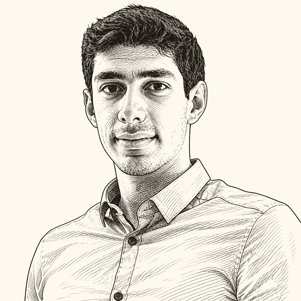
Stanford adjunct professors Shervine and Afshine Amidi argue that training an assistant requires more than teaching a language model to predict the next token. In their account, pretraining builds broad language and code capabilities; midtraining, supervised fine-tuning and preference or reinforcement-learning methods then shape what the model answers and how it behaves. A central challenge is matching each stage’s data and feedback to its goal while controlling costs, long-context demands and the risk of losing capabilities learned earlier.

Pretraining teaches a model to continue, not yet to assist
Shervine Amidi frames large-language-model training as a shift from building a separate model for each task to reusing one model across tasks. In the older setup, spam detection, sentiment analysis, and translation each called for a model trained for that purpose. Transfer learning changes the starting point: first train a model broadly on language, then adapt it for particular uses.
That first stage is pretraining. Its goal is to learn patterns in language and code from a large corpus: web text, multilingual text, software, mathematics, science, and other material. The basic training objective is to predict the next token. A model sees a sequence of tokens and estimates the probability of the next one, then repeats this task across the text.
The prediction can be described one token at a time, but training does not need to proceed sequentially. With teacher forcing, the model receives the known sequence as input and predicts the next token at every position in parallel. The target at each position is the token that actually follows in the training text, regardless of what the model itself predicts. Masked self-attention prevents a prediction from using future tokens: when predicting the token after “teddy,” the model can attend only to “teddy” and the tokens before it. This causal constraint lets training use parallel computation while preserving the information boundary required for next-token prediction.
A student raised a concern about the difference between teacher-forced training and inference: during training, the model is given the correct preceding tokens, while at inference it may have to use its own generated tokens. Shervine Amidi agreed that this creates a mismatch and said the course would return to methods for addressing it. Another question was whether the model receives a prompt at the beginning of a training sequence. In this setup, it does not necessarily receive a meaningful prompt; given only a beginning-of-sequence token, it learns which tokens are likely to start a sequence. The training objective is prediction over text, not yet a user asking a question and receiving an answer.
The cross-entropy objective follows from the probability of a sequence. By the chain rule, the probability of a token sequence is the product of each token’s probability conditioned on the preceding tokens. Maximizing that product is awkward numerically, so the objective takes its logarithm, turning the product into a sum. Training conventionally minimizes the negative log probability, averaged over the number of tokens:
Here, is the target token, the preceding tokens, and the probability assigned by the model. The point of the derivation, Amidi emphasizes, is not to memorize the formula: it is the negative log-likelihood of the training data under the model.
Just think of it from first principles. It’s just you trying to find parameters theta that maximize the probability of your model seeing the training data.
Cross-entropy values depend partly on the tokenizer. A different tokenizer may divide the same text into a different number of tokens, making raw values harder to compare. Bits per byte rescales the loss by the number of tokens and the number of bytes, and converts from nats to bits. Amidi presents it as a way to make comparisons less dependent on tokenizer choice.
Pretraining data is not simply “everything on the internet.” The lecturers describe a large and carefully assembled mixture. Web-scraped sources such as Common Crawl and Wikipedia can supply broad language and knowledge; repositories and sites such as GitHub and Stack Overflow contribute code; math and science material can support capabilities that receive more emphasis in later training. The corpus can reach trillions of tokens. As a scale example, the lecturers cite GLM-5 as having been pretrained on about 30 trillion tokens.
How much of a fixed dataset should be repeated is also a training choice. A chart from Muennighoff and colleagues, shown in the lecture, plots final test loss against tokens trained on and compares repeated data with a prediction for new data. Its annotation says that repeating data for up to roughly four epochs can be almost as good as new data, while returns diminish rapidly after that; at around 40 epochs, the chart labels repetition as worthless. The point is conditional: when data is constrained, another pass can still help, but the value of repeating depends on what new data is available and what quality it has. Repetition is not a substitute for an indefinitely growing supply of useful examples.
Data quality and model architecture can be difficult to disentangle. The lecturers point to DataComp-LM as an effort to study dataset quality while controlling the model-training setup. Without that kind of control, a performance difference could reflect an architecture choice rather than the data. They also describe work that trains small proxy models on different mixtures, fits a regression model to their results, and uses it to estimate promising mixtures at larger scale. Choosing proportions of web, code, or curated sources is an empirical problem, not a fixed recipe.
The preparation itself can involve extraction, filtering, deduplication, language classification, topic and quality classification, and resampling selected material. An Olmo 3 pipeline shown in the lecture begins with sources such as Common Crawl, academic PDFs, and GitHub repositories, then runs them through extraction, filtering, deduplication, and classification before mixing the resulting data. The quantity of source text alone does not make a useful training corpus. Data construction is a substantial process in its own right.
The lecturers also raise a problem that becomes more pressing as generated text spreads online: model collapse. Their explanation begins with finite sampling. Even if a model were perfect, a finite sample from a diverse distribution may miss some rare, long-tail examples. A model is also an approximation, so its output distribution will not reproduce the training distribution exactly. If generated outputs are then fed back into future training, common patterns can be overrepresented while rare ones are underrepresented; the tail shrinks over successive rounds. The lecture adds that preferences inserted by providers and experts can further upweight particular expressions, with examples such as “load bearing” and “byte identical.” Filtering, quality classification, and careful curation are presented as ways to address this risk.
Pretraining and midtraining share the same next-token objective, but differ in what the model is shown and what the training is meant to emphasize. Pretraining builds broad exposure to language and code, often from a very large and mixed corpus. Midtraining continues next-token prediction while shifting toward higher-quality, more task-relevant material. A model intended to handle code or reasoning, for example, can receive more code, mathematics, and science. The objective is still to predict the next token; the data distribution changes.
The GLM-5 material shown in the lecture presents separate stages and figures. One visual labels a general pretraining corpus as 18T tokens at 4K and a code-and-reasoning corpus as 9T at 4K. Another labels long code and reasoning data as 1T at 32K, followed by long-context and agent data as 500B / 50B at 128K / 200K. Elsewhere, the lecturers give about 30T tokens as a summary figure for GLM-5 pretraining. These figures appear on distinct slides, and the source does not explain how they relate; they are best retained as separately reported quantities rather than combined into a reconciled total.
Midtraining may also introduce longer sequences. Standard pretraining commonly uses sequence lengths of several thousand tokens, while actual inputs may run into tens or hundreds of thousands. The GLM-5 example moves from 4K to 32K, then to 128K or 200K in the longer-context stages. The goal is not simply a larger context-window setting, but training that helps the model use information over longer distances.
Long-context training is not just a matter of raising a context-window setting. RoPE provides positional information through rotations, but a model trained on short sequences has not encountered the same position ranges it will see at much longer lengths. Shervine Amidi says that, without additional training, a model may be confused by these unseen rotations. The lecture describes extension methods such as YaRN, which adjust or interpolate RoPE frequencies so longer position differences fall into ranges more familiar from training. It also describes curriculum learning that increases sequence length in stages—for example, 4K, 32K, 128K, and potentially 1M tokens. The GLM-5 example plans the target lengths in advance and uses tweaked frequencies for long-context training and inference.
The obstacle is both computational and data-related. Vanilla self-attention has quadratic complexity in sequence length, so moving from a few thousand tokens to hundreds of thousands sharply increases computation. The lecture also notes that serving systems matter: the training method must ultimately support the way long inputs are handled at inference. Useful long-range examples are not easy to come by, either. A model must learn to use information far earlier in a sequence to make a later prediction, which requires observations where that dependency matters rather than merely a long document. Constructing such observations is a challenge in its own right.
These stages require substantial time, infrastructure, and money. They also leave the model with knowledge tied to the training data and its cutoff. The lecture uses GPT-4 Turbo’s displayed April 30, 2024 cutoff as an example: information about later events was not in that training data. Knowledge can be difficult to update, and the lecturers also list plagiarism among the challenges associated with learned content. These are costs and limitations of acquiring knowledge through training, distinct from the costs of extending context length.
Most importantly, a pretrained model is not automatically an assistant. Asked, “Can I put my teddy bear in the washer?”, it might continue with a plausible passage about what teddy bears are made of, because it learned to complete text rather than answer a user’s question. The answer is consistent with the objective; it is not useful for the intended interaction. The next training stage changes that behavior.
Supervised fine-tuning supplies the desired response pattern
Supervised fine-tuning, or SFT, trains the model on examples of the behavior it should produce. For an assistant, those examples pair prompts or instructions with desired answers. The training objective remains next-token prediction, but now the prompt is context and the target is the answer. The model is not penalized for failing to predict the prompt; the loss applies to the output tokens.
In an instruction-tuning example, the prompt might ask for a short story about a teddy bear that likes poetry, or ask why a teddy bear is a good friend. More generally, SFT data can include assistant dialogues, synthetic instructions, math, reasoning, code, and safety-related examples. It can be human-written or synthetic. Its scale is much smaller than pretraining: the lecture gives thousands to millions of examples, depending on how broad the behavior is meant to be.
The distinction between the prompt and response matters to the training objective. The prompt is already given to the model; the desired continuation is what it is asked to predict. For an input and answer tokens , the conditional prediction is . Shervine Amidi clarifies in response to a question that the model is not trained to predict the prompt itself. The loss is applied to the answer tokens because the aim is to teach the model how to respond.
That difference separates SFT from midtraining. Midtraining still feeds the model a corpus and asks it to predict the next token, with an emphasis on higher-quality or more relevant material. SFT instead uses prompt-and-response examples to tune behavior: given this instruction, produce this kind of answer. In the lecturers’ framing, midtraining changes what the model sees; SFT supplies examples of how it should answer.
The approach creates its own constraints. The model can imitate the examples closely, so the data needs to be high quality. If the prompt distribution overrepresents one kind of request, the model may become biased toward that pattern. Generalization and evaluation remain difficult. The lecturers emphasize that the examples need to reflect the behavior intended by the people training the model; having a large number of examples does not by itself ensure that the model generalizes as intended.
There is a practical cost to updating all the weights of a very large model, especially when the aim is to steer behavior and the model already contains broad knowledge. Low-Rank Adaptation (LoRA) addresses this by keeping the pretrained weights, , and learning an update represented by two smaller matrices, and :
The lecture describes these low-rank matrices as a way to reduce the number of trainable parameters, often with roughly similar performance, depending on the task and data. They also make task-specific storage cheaper. A shared set of base weights can be paired with separate small updates for spam detection, sentiment extraction, or translation, rather than storing a complete model for each task. The base model is reused and the task-specific update carries the change.
The original LoRA paper applied the method to matrices in self-attention. Shervine Amidi says later practice also applies it to the feed-forward network, where much of the model’s compute and many of its parameters reside. LoRA is especially useful for specific tasks or constrained hardware; the lecturers distinguish that case from a general-purpose assistant, which would not ordinarily require a different set of weights for every incoming question. When asked why users do not simply fine-tune all the parameters, Amidi points to practical hardware limits and the fact that the model already has much of the knowledge needed. In that account, changing every parameter is often unnecessary when the aim is a narrower adjustment.
Preference data adds a way to say what the model should avoid
SFT examples show the model what to do, but do not directly provide a negative signal about an answer that is undesirable. A model asked for an activity to do with a teddy bear might say, “I’d suggest you do not spend much time with your teddy bear at all.” It has responded, but not in the way the user wants. Preference tuning adds comparisons between candidate answers.
The lecturers’ case for pairwise comparisons is practical: people often find it easier to say which of two answers is better than to assign an absolute score to one answer. Preference data can also be pointwise, with a score for each response, or listwise, with several responses ranked. Shervine Amidi says pairwise data is the common choice for simplicity. A pair consists of the same prompt and a preferred, or winning, response alongside a less-preferred, or losing, one.
Pairwise preference training is also described as less sensitive to prompt distribution than SFT. That does not mean prompt choice is irrelevant: the comparisons still concern particular prompts and answers. But the lecturers contrast it with SFT, where too much data concentrated on one kind of prompt can make the model biased toward a particular response pattern. Preference data addresses a different problem by directly comparing outputs, rather than requiring a human to write an ideal answer from scratch.
Preference judgments can also expose problems upstream. If the model behaves badly, that may reflect an unintended pattern or low-quality examples in the SFT data. Preference tuning is not a substitute for examining that data; the bad behavior can be a reason to check it. The lecture contrasts the relative ease of judging “A is better than B” with the harder task of generating an ideal answer from scratch. Pairwise collection, however, still requires reliable judgments about what matters.
In RLHF—Reinforcement Learning from Human Feedback—the first stage trains a reward model to score a response to a prompt. The second stage uses those scores to change the language model’s behavior. The “human feedback” is in the preference judgments used to train the reward model; the reward model then supplies scores during alignment. The process has two linked stages: first distinguish good answers from bad ones, then use that distinction to adjust the language model.
The lecture introduces the Bradley–Terry formulation for modeling pairwise preferences. If responses and receive rewards and , respectively, the probability that the first is preferred over the second is modeled as a sigmoid of their reward difference:
The rewards matter through their difference: the formulation models a comparison between two responses, not an absolute probability that one response is good in isolation. A reward model is trained so that the preferred response receives a higher score than the less-preferred one. With a winning response and losing response for a prompt , the objective minimizes the negative log probability assigned to the winning response being preferred:
The derivation starts from the desired comparison: the model should assign a higher score to the winning answer than to the losing one. The Bradley–Terry formula turns the reward difference into a preference probability; taking the log and minimizing its negative gives a training loss. The equation expresses the comparison over preference data, not an absolute score that must be meaningful on its own.
The reward model can use a pretrained language model with a classification head, or an encoder-only model that projects a representation—such as a [CLS] representation—into a score. The lecture cites an example with roughly 10,000 human-labeled observations for reward modeling. The architecture can vary; its role is to map a prompt and response to a quantitative reward that can distinguish preferred from less-preferred answers.
In the second RLHF stage, the SFT model generates responses to prompts, and the frozen reward model scores them. Reinforcement learning updates the language model—not the reward model—to favor outputs with higher scores. The objective balances maximizing reward against staying near a reference model, usually the starting SFT model. That constraint matters because the reward model is imperfect. If the language model optimizes its score too aggressively, it may learn to exploit weaknesses in the reward model rather than become better by the user’s standards. The lecture calls this reward hacking and presents limiting deviation from the reference as one protection against it. It gives roughly 100,000 observations as a scale for this stage, with scores supplied by the reward model.
The reference-model penalty is not an incidental extra term. It constrains how far optimization moves from a model that already knows how to answer and helps guard against over-optimizing an imperfect score. The lecture postpones the mathematical details of the reinforcement-learning update, emphasizing which model is fixed and which is being changed: the reward model stays fixed, while the language model’s weights are updated.
Direct Preference Optimization (DPO) offers a supervised alternative. Rather than first training a separate reward model and then running reinforcement learning, DPO works directly with preference pairs. Its objective is related to the Bradley–Terry loss, with reward expressed through the log-probability ratio between the model being tuned and a reference model. In the lecturers’ explanation, this objective encourages the tuned model to raise the winning response’s probability relative to the reference and lower the losing response’s probability relative to the reference.
The practical contrast is not simply “complicated” versus “simple.” RLHF requires a reward model and a reinforcement-learning stage, with associated models, data, and implementation choices. DPO is supervised and does not need a separate reward model. But DPO trains on fixed responses, not necessarily outputs generated by the model being tuned. The lecturers call this off-policy: the training examples are not the model’s own current outputs. RLHF, in the version described, uses generated responses and is on-policy. The cited comparison says there is no common absolute performance consensus; results vary by task and implementation.
The difference matters because the two methods receive their learning signal in different ways. RLHF generates an output, scores it with the reward model, and uses that score to update the model. DPO compares fixed winning and losing responses from the preference data. DPO’s direct use of preference pairs avoids the separate reward-model stage, but it does not train on the model’s own generated outputs in the same way. The teddy-bear example makes the intended behavioral effect tangible: after preference tuning, the answer shifts toward a friendlier formulation—“It’s better not to. Your teddy could get hurt! A gentle hand wash is safer.”
Reasoning training uses answers that can be checked
? afshine-amidi defines reasoning simply as the ability to solve a problem. A question asking for a course code tests whether the model has the relevant fact. A question asking how old a bear born in 2020 is requires a calculation using the current year. The latter is the kind of task reasoning training targets.
Chain-of-thought prompting demonstrated one way to elicit reasoning: examples show a model explaining steps before giving an answer. The limitation, as Afshine Amidi puts it, is that users should not have to instruct the model to reason every time. Reasoning models aim to produce that behavior through training.
For coding and mathematics, a key advantage is that many answers can be verified. Code can be run against test cases; a math answer can be compared with a known result. This allows training to use a verifiable reward—for example, whether the final answer is correct—and potentially whether the response includes a reasoning chain. The reward is coarser than a token-by-token assessment: an entire response may be marked right or wrong.
The lecture describes Group Relative Policy Optimization (GRPO) at a high level. Given a prompt, the policy model generates several candidate responses. The setup uses rewards for those responses and computes each response’s advantage relative to the group. Responses that perform better than their peers are encouraged; weaker ones are discouraged. The objective also limits deviation from a reference model. For reasoning tasks with verifiable answers, rewards can come from checking an outcome against the ground truth rather than training a separate human-preference reward model.
The GRPO diagram makes the group comparison central: one query produces several outputs, the rewards for those outputs feed a group computation, and the resulting advantages guide the policy. The reference model supplies a constraint against moving too far from the starting behavior. This keeps the broad optimization pattern familiar from RLHF—promote higher reward while limiting drift—but changes where the reward comes from. In the reasoning example, correctness can be verified directly.
The lecturers show two DeepSeek-R1-Zero training curves: accuracy on a reasoning benchmark rises over training steps, and average response length rises as well. They use the charts to illustrate what was observed during reinforcement learning. The figures show concurrent upward trends; they do not establish that longer traces caused the accuracy improvement. The mathematical details of GRPO are left for a later session.
There is a cost to relying on sequence-level correctness. A response may be judged entirely right or wrong even when its intermediate reasoning contains useful or faulty steps. Meanwhile, SFT supplies dense token-level supervision, but on examples that were not generated by the model. The lecturers describe the contrast as off-policy data that is dense but not from the model, versus on-policy rollouts that come from the model but often receive a sparse sequence-level reward.
On-policy distillation is presented as an attempt to combine those advantages. The student model generates its own response to a prompt, and a stronger teacher evaluates the student’s trajectory token by token. Instead of only rewarding or penalizing the completed sequence, training compares the student’s predictions with the teacher’s conditional predictions along the student-generated path. That makes the supervision both on-policy and dense: it follows the student’s own output, while supplying feedback at individual token positions.
| Training approach | Where the sequence comes from | Feedback described by the lecturers |
|---|---|---|
| SFT (off-policy) | Fixed examples, not generated by the current model | Dense, token-level targets |
| Preference or reasoning RL (on-policy) | Responses generated by the model | Often sparse, sequence-level reward |
| On-policy distillation | Responses generated by the student model | Dense, token-level teacher predictions |
If a separate teacher is unavailable, on-policy self-distillation can use the same model in a teacher role. The lecture describes using the same model with a result to steer its response. Another variant uses multiple specialized teachers—for example, models focused on mathematics or software engineering—to transfer capabilities into a student through dense supervision. In each case, the student-generated trajectory supplies the path on which the training signal is evaluated.
The lecturers describe reasoning traces as part of the model’s output, even when hidden from users. They take up output tokens and can count toward API costs. Afshine Amidi discusses reasons providers may restrict access to full traces: they can expose information about a user or conversation, create security risks, and give others valuable training material. He refers to research presented in the lecture concerning recovery of reasoning traces from some third-party APIs, framing the issue as a potential privacy and security concern rather than a claim about every provider.
That output also has practical consequences for usage. Amidi notes that reasoning tokens may be billed as output tokens even when they are not visible in an API response. A user with a finite budget may therefore pay for both the answer they see and hidden reasoning tokens. The amount of reasoning can depend on model training and settings such as “thinking effort”; he also says models may be trained to use more or less effort depending on the prompt.
GLM-5 illustrates how the stages fit together
To make the training stages concrete, the lecturers use GLM-5, drawing on its technical report and the training details presented in class. They first place it among open-weight models using the Artificial Analysis Intelligence Index. Shervine Amidi describes the index as an aggregator of benchmarks that reduces performance to a single comparative number. He notes that open-weight models are often behind closed models at the frontier, while their technical reports can reveal more of the training recipe.
In the GLM-5 pretraining material shown in the lecture, web data provides general language and common knowledge. The slide describes general language as coming from web data and common facts as naturally included, with classifiers used for the long tail. Common Crawl and similar sources require filtering; the data-preparation examples show extraction, filtering, deduplication, classification, and mixing as parts of the process. Wikipedia and other authoritative sites can supply widely established facts, while less common knowledge may call for more deliberate curation. Code comes mainly from GitHub and other platforms, with special attention to programming languages that are less represented. Higher-quality books, papers, and webpages focused on mathematics and science contribute reasoning-related material.
Shervine Amidi describes the filtering of web material as substantial. Common Crawl covers a broad range of internet content, including material affected by AI-generated text, and heuristics are used to trim the collection. He gives an approximate figure of 1% of inputs remaining after such filtering. The material shown also distinguishes common facts, which may appear naturally in web data, from long-tail knowledge that calls for classifiers and more deliberate selection. The point is not that one filter solves data quality, but that broad web sources are transformed before they become a training mixture.
The lecture presents several GLM-5 scale figures across separate visuals. One slide lists a general pretraining corpus of 18T tokens at 4K and a code-and-reasoning corpus of 9T at 4K. Another labels long code and reasoning data as 1T at 32K, followed by long-context and agent data as 500B / 50B at 128K / 200K. Elsewhere, the lecturers give about 30T tokens as a summary figure for GLM-5 pretraining. The source does not explain how these figures relate, so they should be read as separate reported quantities rather than combined into a definitive accounting.
The training material describes coding tasks that pair issues with relevant file diffs, long-form papers and books, and synthetic multi-turn or reasoning examples. The stated goals include improving general long-context performance and handling “needle-in-a-haystack” situations—finding a relevant fact embedded in a long input. Amidi adds that synthetic examples can place a fact in the middle of a sequence and require the model to use it later. These examples address the data challenge described earlier: long inputs alone do not necessarily teach the model to use distant information.
During ordinary pretraining, data may be concatenated and chunked to fill the context window, so documents can be cut at boundaries. The GLM-5 visualization instead shows midtraining with best-fit packing: the process tries to fit whole documents and pads where necessary, while retaining next-token prediction. The change in packing is a training detail rather than a new objective. Longer sequences and longer documents change the input regime; they do not, by themselves, change the prediction target.
SFT then shifts from predicting every token in a corpus to predicting the desired assistant response. The GLM-5 material shown in the lecture lists general chat—including Q&A, role-play, translation, and long-context interactions—as well as reasoning, scientific and mathematical problems, coding, and tool use. It also describes “think” tokens that let the model reason before answering, and curation filters. In this example, the loss is applied to the assistant’s answer rather than the user’s input.
The final reinforcement-learning phase is divided in the GLM-5 material into reasoning RL, agentic RL, and general RL. Reasoning RL uses mathematics, science, code, and tool-integrated reasoning tasks with checkable outcomes. Agentic RL places the model in an environment where actions can be tested—for example, fixing a bug until a failing test passes. General RL addresses less mechanically verifiable qualities such as foundational correctness, emotional intelligence, and task-specific quality, where expert judgment enters. These categories use different sources of feedback: answer checks, task outcomes, and judgments about qualities that are less easily reduced to a single test.
Optimizing distinct objectives across these stages can cause previously acquired capabilities to degrade. The lecture describes GLM-5’s use of on-policy cross-stage distillation as a way to address this risk: later-stage training can use earlier checkpoints as teachers, helping preserve capabilities from SFT and previous RL stages. The source presents this as a response to catastrophic forgetting, not as a guarantee that every earlier capability is retained.
Open reports do not necessarily disclose every part of a training mixture. The lecturers caution that reports may omit some sources and mention public allegations that companies have used other models’ outputs for training. They present this as a reason to read technical accounts critically, not as a settled description of any particular model’s recipe.
The lecturers also briefly connect reasoning training to deployment. Shervine Amidi points to the coding agent Pi as an example of a minimal harness and relates its design to models trained to understand coding-agent tasks without requiring a very long system prompt. The cited author’s account suggests that extensive reinforcement-learning training can make a model understand what a coding agent is expected to do. The lecture presents this as one possible consequence, not as a demonstration that harness design no longer matters.