The O(4) Mass Gap Scales as √βe⁻πβ at Strong Coupling

In the two-dimensional O(4) model, each lattice site carries a unit vector with four real components. Neighboring spins prefer to align. The question in OpenAI’s September 23, 2026 manuscript, “Sharp mass bounds for the two-dimensional O(4) model,” is how long a local fluctuation can remain detectable.

The manuscript defines a lattice mass gap through a transfer operator: an operator that advances the system by one lattice step. The equilibrium state—the vacuum—is removed, and the norm of the remaining operator is converted to a decay rate by taking its negative logarithm. The parameter $\beta$ is the inverse coupling; larger $\beta$ means stronger alignment between neighbors.

The word full matters. A gap measured only through correlations of a single spin component could miss slow behavior in observables unchanged by a common rotation. A neighboring-spin dot product, or bond energy, is one such observable. The claimed gap therefore covers the full local-observable spectrum, including rotation-invariant sectors, not just a selected spin correlation.

For sufficiently large $\beta$, the manuscript claims that this full gap lies between fixed positive multiples of

The constants do not vary with $\beta$. This is a sharp order bound, not an exact asymptotic prefactor. The paper also claims a positive full gap at every finite positive $\beta$, and a unique local limit of periodic square lattices. It does not claim uniqueness for every possible non-periodic Gibbs state.

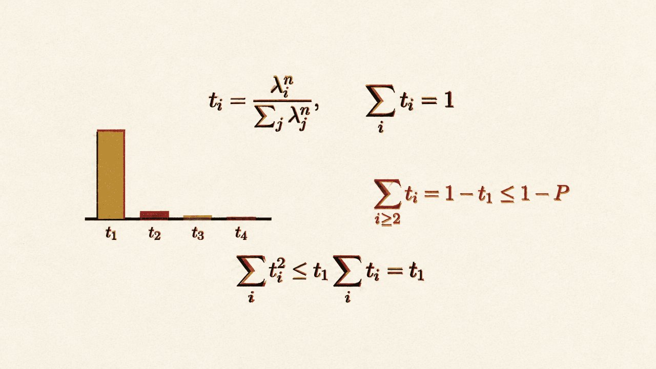
The proof’s bridge from finite boxes to long-distance behavior begins with a cylinder of fixed circumference. Its positive transfer operator has non-negative eigenvalues, with one largest eigenvalue. Closing the cylinder after $n$ steps gives a partition function equal to the sum of the eigenvalues raised to the $n$th power. Normalize those terms into weights $t_i$, which add to one, and define their purity as ${\sum }_i{t}_i^2$.

Because every weight is no larger than the largest one, each squared weight is at most the largest weight times that weight. Summing gives

If purity is close to one, the largest weight must be close to one too, leaving little total weight in all the other sectors. This controls the combined excited weight—including multiplicities and rotation-invariant sectors—without identifying an individual mode.

A single circumference would not suffice: a wider system might contain new slow modes. The manuscript tests periodic rectangles in both directions using a partition-function defect,

The area-proportional bulk contribution cancels exactly. Positivity of the transfer operator connects this defect to spectral weights across the two dimensions. Splitting the enlargement into an $n$-by-$n$ to $2n$-by-$n$ step and then a $2n$-by-$n$ to $2n$-by-$2n$ step yields non-negative terms $p$ and $q$, with ${\Delta }_{\beta }(n)=2p(n,n)+q(2n,n)$.

Once the defect is at most $2^{-10}$, doubling the side gives a next defect no larger than $64{\Delta }_{\beta }(n{)}^2$. This is an estimate on the defect, not by itself a mass-gap bound. The manuscript combines its decay under repeated doubling with further rectangle identities that relate the defects to spectral weights. It then uses an infinite-volume passage to obtain the claimed lower bound: in every local limit of these doubled periodic squares, the full gap is at least $\log 2/n$. The rectangle identities and passage to the local limits are essential steps between the finite-box estimate and that conclusion.

The hard part is making the finite-box test small at the right length. A preliminary mixing estimate supplies a reference box, but its length is too large to yield the sharp scale. The paper then groups spins into blocks using an exact probability kernel. This integrates finer spins while retaining extra interactions and rough configurations; it is not simply a replacement of each block by its average.

To compare different blocking depths, the manuscript matches their terminal kinetic coupling. On admissible boxes and at sufficiently large depths, it compares the complete positive densities after extracting bulk area factors. The comparison holds on a common set of high probability under both laws and preserves the box test. This allows the proof to fix a reference depth and coarse box while continuing to refine the microscopic cutoff.

The factor $\sqrt{\beta }$ comes from calibrating the blocking drift. If $L$ is the fixed blocking factor and $N$ the number of steps, the paper obtains

where $R$ stays bounded. Exponentiating the negative gives

Since the remainder is bounded, its exponential contributes only fixed positive factors. The half-logarithm is essential: keeping only the leading exponential would lose the square-root factor. The coefficient calculation and uniform error control are inputs to the proof, not consequences of this algebra.

For the upper bound on the gap, the paper needs a correlation that remains nonzero. At a sufficiently large fixed terminal coupling, it bounds the expected squared difference across each of three neighboring bonds by $1/9$. By Cauchy–Schwarz, the expected squared difference between the endpoints is at most three times the sum of those three expectations, hence at most one.

For unit vectors $u$ and $v$, $|u-v{|}^2=2-2u\cdot v$. The endpoint dot product therefore has expectation at least $1/2$. Rotation symmetry distributes that correlation equally across the four components, leaving at least $1/8$ in one component.

The proof transfers this correlation to conditional means of a component given the original spins. Each mean is a function of the spins in its own ancestral block, has mean zero, and is bounded in magnitude by one. Conditional on the original spins, the auxiliary randomness used to construct the two block variables is independent. Thus the conditional expectation of their product is the product of their conditional expectations. Averaging over the original spins gives the expectation of the product of the two conditional means; by iterated conditioning, that expectation equals the original component correlation. This is the step that preserves the correlation in the block variables.

Their ancestral blocks are separated by at least $L^N$ lattice steps, the scale of $N$ successive blocking steps with factor $L$. The full gap bounds their correlation by $e^{-m_{\mathrm{lat}}{L}^N}$. Combining this with the surviving lower bound $1/8$ gives $m_{\mathrm{lat}}({\beta }_N)\le \log 8/L^N$.

Together with the lower bound from the box test, this yields uniform positive and finite mass bounds when physical units are assigned by fixing a reference length independently of the mass. Uniform bounds for lattice cutoff theories do not themselves construct a continuum limit; that would require convergence of the transfer dynamics and suitable observables.