The Standard Map Has Positive Metric Entropy at Sufficiently Large Parameters
An OpenAI preprint claims that the standard map has positive metric entropy with respect to normalized area for every sufficiently large positive parameter. The theorem means the largest Lyapunov exponent is positive on a set of positive area; it does not claim positivity almost everywhere or give a numerical threshold. The proof controls how stretching can cancel across intervals, then uses those bounds across doubling time scales to rule out zero exponent almost everywhere at arbitrarily large parameters.
The theorem concerns area, not a striking orbit
A complicated orbit of the standard map does not establish chaos on a set of positive area. The manuscript claims that for every sufficiently large positive parameter , the map has positive metric entropy with respect to normalized area. Equivalently, its largest Lyapunov exponent is positive on a set of positive area.
The map acts on a torus, represented as a square whose opposite edges are identified. At each step it changes the vertical coordinate and then the horizontal one:
Both coordinates are taken modulo one. Each operation is a shear with Jacobian determinant one, so their composition preserves area. Stretching in one direction is balanced by compression in another.
For this smooth area-preserving map, the entropy formula identifies metric entropy with the area average of the largest Lyapunov exponent. That exponent is nonnegative, so positive average entropy means it is positive on a set of positive area. The result does not say that exponents are positive almost everywhere, that the whole torus is ergodic, or that entropy has a uniform positive lower bound. The manuscript gives no numerical value for the threshold .
The numerical illustration uses only to show the map’s rule. A few iterates, however complicated, do not establish the theorem. The claim and proof discussed here are in the pinned manuscript.
Derivative growth can disappear when directions cancel
To study stretching, the proof changes coordinates so that the horizontal coordinate at time , denoted , obeys a second-order recurrence:
Small perturbations evolve according to matrices
Their products track derivative growth. The matrices have determinant one. The proof measures the growth of a product from time to time by , with ; this normalization gives .
Large norms on shorter intervals do not guarantee large growth over a longer one, because the directions of stretching can cancel. The source illustrates this with two matrices, each of norm four, whose product is the identity:
| Matrix | Effect | Norm |
|---|---|---|
| A = diag(4, 1/4) | Stretches horizontally; compresses vertically | 4 |
| B = diag(1/4, 4) | Undoes A's stretching and compression | 4 |
| BA = I | The combined transformation is the identity | 1 |
One major estimate addresses cancellation in the actual dynamics: once the parameter is sufficiently large, two long intervals can each have nearly maximal growth while their combined interval almost entirely cancels only with exponentially small probability in the interval length. The bound is uniform in the center and length. Its proof relates expansion scales on either side of the interval and shows that the analytic coincidences needed for severe cancellation are scarce. It treats, among other cases, nearly opposite cosine terms and a phase slope approaching zero.
A second estimate compares weighted observations near opposite ends of a fast-growing bridge. Contracting coordinate graphs and controlled Jacobians provide the bound. It does not assume distant observations are independent, and it applies only under the fast-bridge condition.
Scale doubling measures how cancellation accumulates
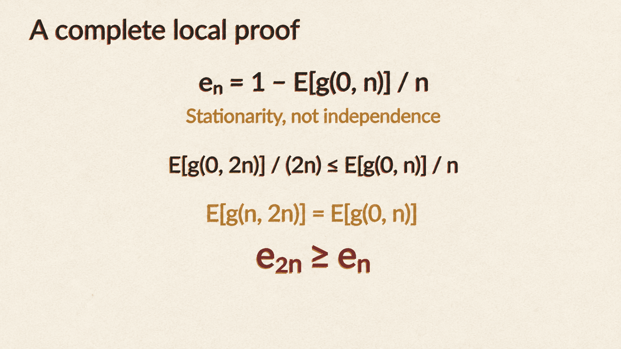
A simpler identity shows how local cancellation enters the larger argument. Let
where the expectation is over normalized area. This is the expected shortfall from maximal growth over steps. Split a product of length into two length- pieces. Since the norm of a product is at most the product of the norms,
Area preservation makes the growth process stationary, so the two halves have the same expected growth. Averaging the inequality and dividing by gives . This uses stationarity, not independence.
The difference has an exact interpretation. Define the cancellation loss
Then
Cancellation therefore increases the expected shortfall as the observation window doubles. The paper’s harder estimates constrain how large these increases can be in the standard map.
The contradiction depends on what the shortfall does across scales
The proof rules out a sequence of arbitrarily large parameters for which the exponent is zero almost everywhere. Under that supposition, two limits pull in opposite directions. For any fixed orbit length , the expected shortfall tends to zero as grows. But at each fixed parameter in the supposed sequence, zero long-run growth forces toward one as the orbit length grows. These are different limits; the proof does not exchange them.
Instead, it chooses a slowly growing starting scale , then follows dyadic scales until a first scale crosses a small, parameter-dependent threshold. Estimates control how much the shortfall can increase at each doubling. The remaining question is whether those increases can add up consistently.
To compare them, the proof records growth between times and rescales time and growth together. The cancellation and bridge estimates restrict the possible limiting patterns: growth can be entirely slow, or there can be a slow region with one or two exterior rays of unit speed. “Slow” does not mean constant speed.
A capped shortfall function then makes the comparison tractable. It assigns a value of one to uniformly slow intervals, while near zero shortfall it grows linearly with a small slope. Averaging it over area, the proof compares a whole interval with its two halves. Summing the signed changes over dyadic scales makes intermediate terms cancel, leaving a positive balance between the starting and terminal scales.
That positive terminal balance records net change in the area-averaged capped shortfall across the selected range of scales. The contradiction is that the terminal-scale contribution is strictly less than this balance, while the integrated invariant remainder is non-positive. Adding those bounds cannot recover the positive total the scale sum requires. Controlling mass near constant-speed patterns is essential: without it, the terminal contribution could not be shown to fall short. Together, the estimates rule out the supposed sequence of zero-exponent parameters.
For every sufficiently large positive , a positive-area set therefore has positive largest Lyapunov exponent, and the standard map has positive metric entropy with respect to normalized area.