Two Limit Cycles Are the Exact Maximum for a Quintic Liénard Class
An OpenAI manuscript proves that a planar Liénard system with restoring force \(x\) and a polynomial damping term of degree at most four can have no more than two isolated periodic orbits, even when degenerate cycles are counted. The result applies to systems whose defining polynomial \(F\) has degree at most five, not to all planar systems with quintic terms. The authors establish the upper bound by comparing orbit halves and counting zeros of a matching function, then construct a small perturbation with two isolated cycles to show the bound is sharp.
Two is the maximum for this Liénard class
A periodic orbit is not necessarily a limit cycle. In an undamped oscillator, every circle around the equilibrium is periodic, but none is isolated: periodic circles lie arbitrarily close to each one. A limit cycle is an isolated periodic orbit.
OpenAI’s manuscript Two limit cycles for quintic Liénard systems proves that the maximum is exactly two for the system †
ẋ = y − F(x), ẏ = −x,
where F is any real polynomial of degree at most five. The count is of distinct geometric images of isolated, non-constant periodic solutions, including degenerate ones. The result is not a bound for every planar vector field with quintic terms.
In the equivalent second-order equation, x″ + F′(x)x′ + x = 0, the restoring force is exactly x and the damping polynomial has degree at most four. F need not be odd; its even coefficients are unrestricted. A vertical shift removes its constant term, and reflection with time reversal lets the proof take the quintic coefficient to be non-negative. These normalizations preserve the number of geometric cycles.
The exact bound combines two different arguments: a global comparison rules out a third cycle, while a local construction produces two.
Matching half-orbit endpoints turns cycles into zeros
For the global bound, the proof divides an orbit into its right and left halves. On either open half-plane, x has a fixed sign, so ẏ = −x is nonzero and has a fixed sign. Thus y changes monotonically and can serve as the coordinate along each half-orbit.
Set u = x²/2. Since u̇ = x ẋ, dividing by ẏ gives du/dy = F(x) − y. On the right half, substitute x = √(2u); on the left, x = −√(2u). Each half-orbit becomes a positive arch in the (y,u) plane, with endpoints at u = 0.
For each arch, let r be half the distance between its endpoint heights and M their midpoint. The endpoints are M − r and M + r. Two arches with the same width r close into an orbit exactly when their midpoints agree. The proof therefore defines
Δ(r) = M₊(0,r) − M₋(0,r).
A closed orbit corresponds to a zero of Δ, and a limit cycle to an isolated zero. The manuscript establishes this correspondence on one common open interval of widths for both arches and checks separately that no cycle is missed at the equilibrium boundary. This reduces the orbit-counting problem to counting isolated zeros of one function.
Comparison theorems constrain the number of zeros
After the coordinate change, the two arch equations share a quadratic part determined by the even coefficients of F. Their remaining terms have opposite signs and are represented by p(u) = e u^(1/2) + c u^(3/2) + a u^(5/2), with a ≥ 0.
The proof compares each actual arch with a quadratic model by fitting endpoint data: the model matches the arch’s midpoint and the midpoint’s derivative with respect to width. It is not a parabolic replacement for the entire arch. A global fitting theorem makes the comparison available at every admissible width. Transport equations track the fitted parameters; the model inequality uses endpoint variation, a Riccati linearization, and a Schwarzian identity.
The resulting bounds depend on the signs of the first two coefficients, e and c, in the odd contribution p; the leading coefficient a is non-negative. The comparison theorems use those sign cases to constrain the fitted-curvature difference and hence the possible zeros of Δ. When e ≥ 0 and c ≥ 0, there are no limit cycles. When e ≥ 0 and c < 0, at most two are possible. When e < 0, either sign of c gives at most one. These bounds include cases where leading coefficients vanish.
Only the case e ≥ 0 and c < 0 can reach two. There, the comparison results show that the difference q(r) between the fitted curvatures is nondecreasing, and give
Δ′ = AΔ + Bq, with B > 0.
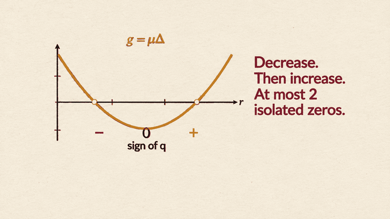
Choose a positive integrating factor μ with μ′ = −Aμ. Then (μΔ)′ = μBq. Since μB is positive, the derivative has the sign of q. The monotonicity of q, together with this sign relation, means μΔ can decrease, flatten, and then increase, but cannot repeatedly reverse direction. It has at most two isolated zeros. A zero interval contributes no isolated zeros.
A local perturbation realizes two isolated cycles
For the lower bound, the manuscript takes Fε(x) = εf(x), where f(x) = 4x − (20/3)x³ + (8/5)x⁵. Start on the positive y-axis at height s, and let P(s, ε) be the height of the first return to that axis. With E = (x² + y²)/2, differentiation along the system gives Ė = −εxf(x). Integrating over the return yields
(P(s, ε)² − s²)/2 = εQ(s, ε).
At ε = 0, x = s sin t. Over one full turn, the integrals of sin²t, sin⁴t, and sin⁶t are π, 3π/4, and 5π/8. Substitution gives
Q(s, 0) = −πs²(s² − 1)(s² − 4).
The positive roots, s = 1 and s = 2, are simple: Q_s(1, 0) = 6π and Q_s(2, 0) = −48π. Smooth dependence and the implicit function theorem continue both roots for the same sufficiently small positive ε.
At either continued root, Q = 0, so P² = s². Since the return height is positive, P = s and the trajectory closes. Differentiating the return-energy identity at such a root gives s(P_s − 1) = εQ_s. The continued roots remain simple, so Q_s is nonzero; hence P_s ≠ 1. The return-map fixed point is therefore isolated, and so is the periodic orbit. The inner cycle repels and the outer attracts. The displayed trajectories at ε = 0.05 are numerical illustrations, not a certified existence threshold.
The construction gives two isolated cycles; the global comparison rules out a third. For the stated class of systems, two is the exact maximum.