Exact Gaussian Labels Still Require d log(1/ε) Samples Under Subquadratic Memory

Suppose an unknown unit vector S must be learned from observations Yₜ = ⟨Xₜ, S⟩, where the Xₜ are independent standard Gaussian vectors. The labels are exact: there is no measurement noise. Each observation constrains S to a slice of the sphere, but a streaming learner cannot retain all the observations. It must compress what it has seen into a memory state of at most M bits, while computation on the current observation is unrestricted.

The manuscript’s streaming theorem gives a sample lower bound for this setting. If S is uniform on the unit sphere in dimension d, and the learner must estimate it to angular error at most ε with probability at least 3/5, then subquadratic memory, M(d) = o(d²), requires T(d) ≥ c d log(1/ε(d)) for every accuracy sequence 0 < ε(d) ≤ 1/10, once the dimension is sufficiently large. The constant c is absolute; the dimension threshold may depend on the memory sequence. This is a lower bound under subquadratic memory, not a characterization of what is possible with larger memory. It concerns samples, not computation time: even with exact labels and unrestricted computation on each current pair, finer accuracy has a logarithmic sample cost in this regime.

The proof’s central obstacle is selection bias. Before a memory message W is known, the rows that helped produce it have their original Gaussian law. After conditioning on W, they need not. A message that records whether a row’s first coordinate is positive, for example, leaves only positive values of that coordinate when the message says yes. Replacing those rows with fresh Gaussian ones would therefore change the experiment in a way the proof must control.

Rather than treating the rows that formed W as fresh, the argument keeps the joint law of the signal S and message W fixed, and changes the auxiliary observations around that pair. In the aligned experiment, the revealed rows include A, which helped produce W, and independent rows C. In the fresh experiment, the rows G are independent of (S, W). Both experiments reveal rows and their exact labels; these auxiliary observations are for the proof, not for the learner.

With m = ⌊d/10⌋ actual rows and ℓ = ⌊d/2⌋ rows in total, Theorem 4.1 bounds the information W carries about S after the fresh observations are revealed. For countable W with entropy at most d² nats, the fresh-experiment information is at most the aligned-experiment information plus Kd, for an absolute K in sufficiently large dimension. This is a one-sided bound, not an equality.

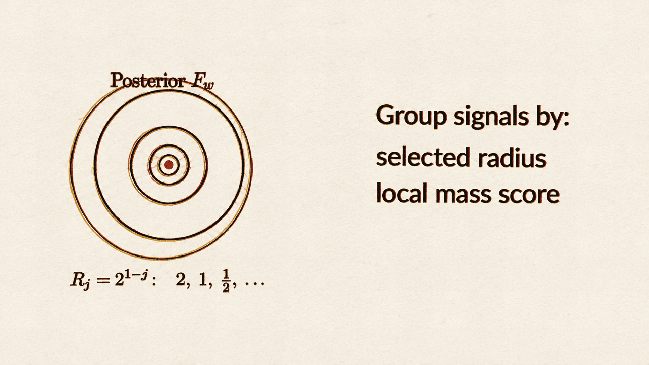
The proof makes the comparison by grouping signals according to the local geometry of their posterior distribution given W. It considers balls around each possible signal at radii 2, 1, 1/2, and so on, and selects the first radius R maximizing posterior mass divided by R to the power ℓ. It also records the rounded-up logarithm Q of that maximum. Signals with the same selected radius and score form a class, and the posterior is normalized within each class.

The key counting step is that, within a class, centers more than 2R apart have disjoint radius-R balls. Each ball has original posterior mass at least e^(Q−1)R^ℓ. Since their total mass cannot exceed one, the number N of centers is at most e^(1−Q)R^(−ℓ). Maximality means the corresponding doubled balls cover the class: if a point were left uncovered, another center could be added.

This cover bounds the fresh experiment’s continuous-label entropy. Revealing which covering ball contains the signal costs at most log N; within a ball, the signal is within 2R of its center. The entropy bound contributes a term ℓ log R, canceling the radius term in the cover cost and leaving −Q plus a term of order d. On the aligned side, a high-moment bound on expected log density gives a corresponding +Q term. Averaging over the refined classes cancels these terms. That cancellation is what prevents the local posterior geometry from accumulating into a larger cost: with moment order ⌊d/10⌋ and entropy H(W) ≤ d², the remaining refinement costs yield an information gap of order d.

The comparison applies to successive blocks of observations. Let U be the memory before a block and W the memory after it. In the aligned experiment, conditioning on the block data leaves the update as a randomized channel from U to W, with no further access to S. Conditional data processing then prevents the update from increasing information about S. Replacing the block’s observations with fresh ones costs at most Kd.

The resulting fresh-row information potential starts at zero and grows by at most Kd per block of roughly d/10 samples. After T samples, it is bounded by a quantity proportional to d⌈T/m⌉.

Success requires more when ε is small. Conditioned on the auxiliary Gaussian equations, S lies on a residual sphere of roughly half the original dimension; its radius is at least 1/2 with high probability. The proof compares the actual learner with a reference law that preserves the relevant conditional marginals but makes the remaining signal and final memory state independent given the side data. The output rule is the same under both laws.

Under that reference law, a fixed output can match only a small cap of the possible signals. On the event that the residual radius is at least 1/2, the cap probability is at most (4ε)^(d−ℓ−1). Since the actual learner succeeds with probability at least 3/5, the divergence between the actual and reference laws must be at least c₀d log(1/ε). Comparing this required information with the blockwise upper bound gives the stated sample lower bound.

The manuscript separately handles stopping, independent rule seeds, and the final block. Its output restriction allows the terminal state, stopping index, and fresh randomness; the last sample is not an extra memory channel.