Subquadratic Memory Requires More Samples for Higher Gaussian Precision
For the paper’s specified message-alphabet size, an OpenAI preprint bounds the information in \(t\) messages by a constant times \(dt\) in sufficiently large dimension, with the constant depending on the alphabet-size parameter. It uses that bound to show that a one-pass learner with memory \(o(d^2)\) needs at least order \(d\log(1/\varepsilon)\) samples to estimate every unit signal to angular error \(\varepsilon\), with success probability at least \(2/3\), for \(0<\varepsilon\leq 1/10\).
Exact observations do not remove the memory constraint
An observation can be exact and still be hard to retain. In the model analyzed in the OpenAI paper, the unknown signal is a unit vector S. Each new observation is an independent Gaussian vector X, accompanied by the exact inner product of X with S. There is no measurement noise. But the learner carries only a finite persistent state from one observation to the next. Unlimited computation does not make that state an unlimited store of information.
The question is how much information a sequence of finite messages can extract from these observations. Counting the possible messages is not enough: earlier messages change the learner’s conditional distribution over the signal. That changed posterior can concentrate on a small region, affecting what later blocks reveal.
The paper studies this through a carefully chosen prior. Write n = d − 1, draw Z uniformly from a centered n-dimensional cube of side length 1/√n, and form the unit vector φ(Z) = (Z, √(1 − ‖Z‖²)). The prior is uniform in cube volume, not in spherical surface area. Measurements are grouped into blocks of k = ⌊n/16⌋ rows. Each block passes a message from an alphabet of size at most exp(A d²).
For fixed A and sufficiently large d, the manuscript bounds the information in t messages by a constant times d t. The constant may depend on A. This is the central information bound in the paper†. The difficult part is proving it when the posterior changes after each message.
Localization costs information, but its name costs less
To control changing posteriors, the proof lets the analysis reveal a nested dyadic cell containing Z after each message. These are bookkeeping revelations, not extra memory for the learner. They track how localized the posterior has become.
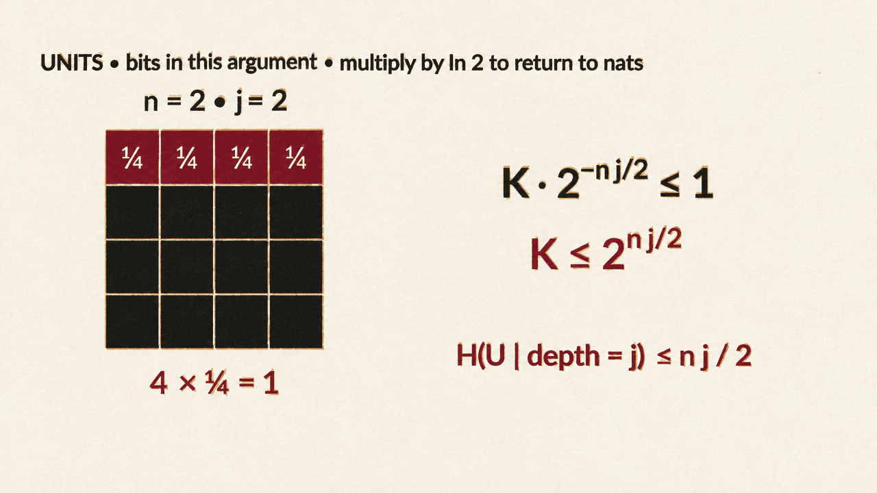
The proof calls the posterior “spread” when no descendant cell has too much probability. If each coordinate has been halved j times, the probability of a cell at that relative depth is at most B · 2^(−nj/2). Here B ≥ 1 is slack: it measures how far the posterior is from meeting the spread bound tightly. Under this condition, a fresh block’s message carries information bounded by a dimensional term, log B, an alphabet-size term of order (log N)/d, and an exponentially small tail. For the stated alphabet, the alphabet contribution is of order d. The remaining task is to pay for restoring spread after a message changes the posterior.
At a fixed depth j, cells are disjoint and their posterior masses sum to one. So if a cell is called heavy when its mass is at least 2^(−nj/2), there can be at most 2^(nj/2) heavy cells. Once the depth is known, naming one costs at most nj/2 bits. Yet being confined to a cell at total depth J certifies at least nJ bits of relative entropy from the original uniform-cube prior: the cell has prior mass 2^(−nJ), and the exact decomposition adds a nonnegative within-cell divergence. The posterior need not be uniform inside the cell.
The proof selects the sampled point’s deepest heavy ancestor, rather than revealing just any cell that contains it. This distinction matters because the probability of selecting a cell is not necessarily the probability of lying inside it. In the source’s small illustrative grid, a region R contains half the probability, while its heavy child contains one quarter. Points in that child select the child, not R; only the remaining quarter selects R. Thus P(Z ∈ R) = 1/2 but P(U = R) = 1/4. The conditional law after selecting R must be normalized by the selection probability. This example illustrates the selection rule; it is not the high-dimensional Gaussian theorem.
The analysis also charges for naming the random depth and for the slack B needed by the next block. It bounds depth entropy by expected depth plus one bit, and expected log-slack by depth entropy plus a constant.
Let J denote the final accumulated localization depth, and let I denote the information in the messages together with all selected cells. Summing the block bounds gives an upper bound of C_A d t + (n/2 + 2)E[J]. Confinement gives the lower bound I ≥ nE[J]. For sufficiently large dimension, subtracting these bounds leaves a positive fraction of n, so E[J] = O(t). Substituting back yields I = O(dt).
| Charge or bound | Quantity |
|---|---|
| Information upper bound | C_A d t + (n/2 + 2)E[J] |
| Information from confinement | At least nE[J] |
| Consequence in sufficiently large dimension | E[J] = O(t), then I = O(dt) |
The Gaussian step links spread to message information
The counting is elementary; connecting spread to the message bound requires the Gaussian geometry. The proof draws independent copies from the posterior and expands a moment of a projection density. Nearly flat simplices can produce large inverse-volume factors. The spread condition controls how likely a new point is to approach the affine span of earlier points, while Gaussian orthogonalization bounds the resulting moment.
The analytic argument allows inserted weights, then uses duality to control message likelihoods. It temporarily smooths the labels and removes that smoothing before applying the result to exact observations. The higher-dimensional moment proof and the weighted-density, limiting, and duality arguments are omitted. The geometric diagram is illustrative, not a proof of those steps.
Subquadratic memory forces a precision-dependent sample count
The information bound applies to a one-pass learner with deterministic finite horizon T and persistent memory M(d) = o(d²). Suppose it must return an estimate with angular error at most ε, with success probability at least 2/3 for every unit signal, where 0 < ε ≤ 1/10. Each block’s message must account for the continuing state or the terminal state and local stopping position; stopping information is not discarded.
Under the cube prior, any fixed guess is ε-accurate on a region of probability at most (5ε)^(d−1). Reliable accuracy therefore requires information of order d log(1/ε). Since t blocks reveal at most a constant times dt information, the learner needs at least order log(1/ε) blocks. Each block contains order d rows. A separate full-data argument handles constant accuracy and block-count rounding, yielding a sample lower bound of order d log(1/ε). The stated dimension threshold may depend on the memory sequence.
The paper also gives other localization routes, with their own assumptions and two information corrections; the argument here is its first complete route. For finite-memory learners, the consequence is that exact observations do not eliminate the cost of maintaining information across a stream: under the stated memory and success conditions, higher precision requires a proportionally larger logarithmic factor in the sample count.