Subquadratic Memory Requires More Samples for Exact Gaussian Direction Estimation

With memory growing more slowly than d² bits, a learner needs at least a constant times d log(1/ε) samples to estimate a uniformly random direction in d dimensions to angular error ε, with success probability at least 2/3. This holds even though each sample gives an exact, noiseless Gaussian measurement. The constraint is that the learner processes each fresh, unchosen sample once, retains only a finite state, and cannot revisit the raw data.

Without that memory constraint, d independent measurements and their real-valued labels determine the direction almost surely by linear algebra. The OpenAI manuscript Posterior replicas and conditional information in Gaussian regression studies what changes when the learner must repeatedly discard its observations. The error level may depend on dimension, but must satisfy 0 < ε ≤ 1/10 radians. The constant in the lower bound is absolute; the dimension from which the result applies may depend on the memory sequence. Computation and randomized updates are unrestricted, and the learner must stop by a deterministic sample horizon.

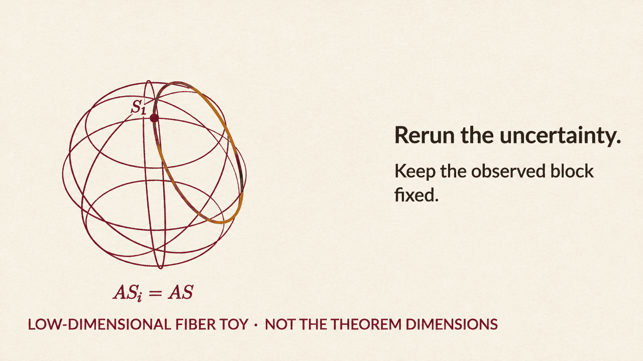
The proof’s central tool is a one-block information bound. A signal S has a Borel probability density bounded by L relative to the uniform distribution on the sphere. A Gaussian matrix A produces exact labels AS, which are compressed into a finite message W. The learner does not see the later side information: an analyst independently receives a Gaussian matrix B and the projection BS.

The quantity being bounded is the conditional mutual information I(S; W | B, BS): how much the message reveals about the signal after the analyst’s projection is known. For the row counts in the manuscript, let k = 2⌊d/16⌋, m = k = t − 1, and l = 4k, where A has k rows and B has l. For sufficiently large d, the manuscript bounds the information by

Here entropy is measured in nats, and C denotes an absolute constant. Since t grows proportionally to d, the message-entropy contribution is divided across a number of replicas proportional to dimension.

Those replicas are independent draws from the posterior distribution of signals compatible with the observed A and AS. They are drawn independently of W given that shared data, so each replica paired with W has the original signal-message law. But after the shared data are hidden, the replicas are dependent: they all satisfy the same observed equations. They are proof devices, not extra samples available to the learner.

If K is the replicas’ total correlation before the projection and K′ their total correlation conditional on B, an information chain rule yields

The proof needs to bound only the dependence lost under projection, not eliminate all dependence among the replicas.

For two distinct candidate signals u and v at distance r, one standard Gaussian row a gives a difference in labels distributed as rZ, where Z is standard normal. Its density at zero is 1/(√(2π)r); for k independent rows, the density is (2π)^(−k/2)r^(−k). Halving the distance multiplies this density by 2^k. This is a density calculation, not a positive probability that distinct signals produce exactly equal labels: for a fixed pair, that probability is zero.

With multiple replicas, the corresponding geometric quantity is affine volume. Arrange their difference vectors as columns of D; the parallelepiped volume is J = √det(DᵀD). The Gaussian factor scales as J^(−k), which can grow large when the differences are nearly dependent. The manuscript constructs an equal-label finite measure before deriving a posterior likelihood, which also includes the common label density. Volume alone is not the likelihood.

The key to the block bound is that the projected calculation contains a matching inverse-volume term. A normalized likelihood test lower-bounds K′, allowing the matching −k E log J terms in the bounds for K and K′ to cancel in their difference. Density comparisons and exceptional-set arguments complete the proof.

To use the block bound repeatedly, the proof conditions on the learner’s current memory state. If state v has probability pᵥ > 0, the signal’s density given that state is Pr(V = v | S = s)/pᵥ. Since the numerator is at most one, this density is bounded by 1/pᵥ. A rare state may therefore have a large density bound, but its cost is controlled on average: the average of log(1/pᵥ) is the state entropy, and concavity controls the average double-logarithmic term. Applying the block theorem state by state and then averaging handles rare states without assuming their individual density bounds are small.

The proof turns this into an information clock. After reductions for randomness and stopping, it keeps the same independent projection B throughout and records the stopping index in a padded state. In the short-horizon case, the horizon is divided into blocks of order d samples. At each block, the conditional information bound charges at most order d, after averaging over the current memory state. Summing those increments gives terminal information at most a constant times the number of samples; the cost of recording the stopping index is included in that bound.

For the lower side of the comparison, revealing BS still leaves uncertainty on a residual sphere of dimension proportional to d. With high probability its radius is not tiny. A small angular target occupies a small fraction of that sphere, so an information inequality makes successful localization cost at least order d log(1/ε). Comparing this terminal-information requirement with the information-clock upper bound forces the sample horizon to be at least a constant times d log(1/ε).

The paper also develops distance-bin, Haar, synthetic Gaussian, and Stiefel-incidence comparisons; the explainer follows the Gaussian replica route. The explainer’s creators say their executable checks cover the displayed constructions and local identities, not the general analytic theorem, and that a full Lean reproduction was not run.

Exact labels can determine the signal if the learner keeps them. Under a finite-state constraint, posterior replicas let the proof measure what the message preserves, even after an independent view of the signal is revealed to the analyst.