Bounded Memory Forces Logarithmically More Samples for Precise Gaussian Regression

With at most A d² bits of memory, an algorithm needs at least c_A d log(1/ε) noiseless Gaussian observations to estimate a random unit vector to angular error ε with probability at least two-thirds, for 0 < ε ≤ 0.1. Here A is any fixed positive constant; the dimension must be sufficiently large, and the positive constant c_A and dimension threshold may depend on A, but not on ε.

The bound is average-case over the uniform target and the algorithm’s randomness. It does not say every individual target is hard, and it does not give a constant uniform over values of A that grow with dimension. Its point is narrower: even exact measurements do not make fine accuracy immediate when the learner cannot keep all the information they contain.

The model makes that constraint explicit. The target S is uniform on the unit sphere in d dimensions. At each step, the learner receives an independent standard Gaussian vector X_t and the exact inner product Y_t = ⟨X_t, S⟩. It reads the pairs once, in order, and retains at most M bits between observations. Computation and independent randomness are unrestricted, but discarded observations cannot re-enter through the output rule. The learner may stop before a fixed finite horizon T; its final unit-vector estimate can depend only on the terminal state, stopping index, and fresh randomness.

With all exact data retained, d independent Gaussian equations determine the vector almost surely. The lower bound concerns a different resource: the finite state that must carry information forward from one observation to the next.

An exact equation constrains the target to a lower-dimensional slice. Tracking the target distribution after conditioning on each raw observation would therefore change the geometry throughout the proof. Instead, the argument keeps the original uniform sphere fixed and measures how much future success can be concentrated in a small region.

Fix the shared seed, a sample index, and a memory state, whether or not the algorithm actually reaches that state. Let h(S) be the probability of eventual success for target S when the algorithm starts from that state and uses fresh future samples. This is a success function, not a posterior distribution. The proof bounds its mass in every sphere-centered ball of radius r by a quantity of the form (Rr)^a, where a = (d − 1)/2. R is a scale parameter in the bound, not the radius of the function’s support.

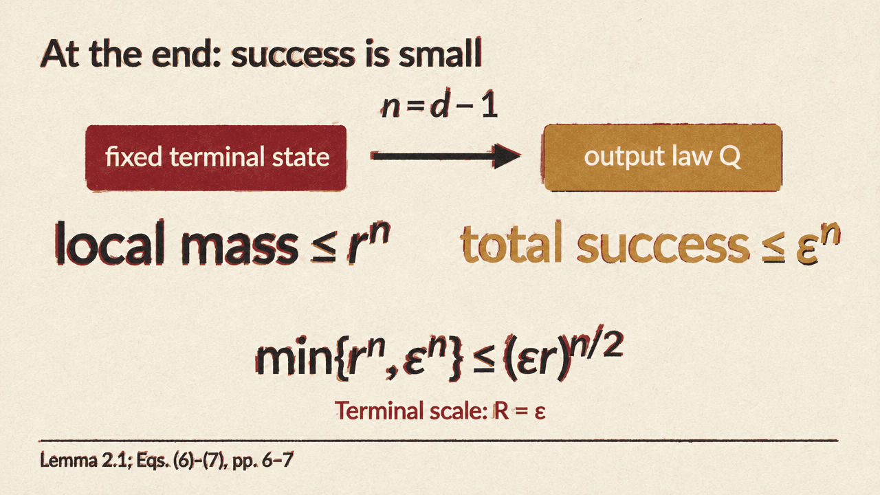
At the terminal state, fixing the seed and stopping index fixes the output rule’s distribution. That rule does not take the unknown signal as an input. A sphere-centered ball of chordal radius r has uniform mass at most r^(d−1), and angular error at most ε implies chordal error at most ε. Thus total successful mass is at most ε^(d−1), even when the output is randomized.

The proof combines this total-success bound with the local bound. For a ball of radius r, it uses the tighter of the two estimates, then bounds their minimum by their geometric mean. This initializes the invariant at scale R = ε. The terminal estimate’s limited success is therefore the starting point for reasoning backward through the states that could have preceded it.

To move backward, the argument groups roughly d observations into a block and gives the block all its exact data at once. This only strengthens the learner. Each possible destination state has its own future-success function, and the proof controls how much successful mass for that state can lie in the same radius-R ball.

Two estimates make the block bound work. One controls how concentrated the successful target mass can be after the block’s Gaussian rows and labels are mapped into data space. The other bounds the average volume of the projected region those labels can occupy. In the proof, this region is a common ellipsoid determined by the projection. The concentration estimate loses a power of the radius, while the volume estimate restores that power through Hölder’s inequality. The projection argument relies on inverse distances to affine spans and Gram determinants.

The remaining cost is selecting a destination. With N possible destinations, the mass bound incurs a factor N^(1/q), where q is proportional to d. Converting that mass bound back into a bound on the scale R requires taking a root of order a, also proportional to d. Thus the state count contributes an exponent proportional to 1/d, and taking the root contributes another factor proportional to 1/d: together they make the scale cost depend on 1/d². For a block of m observations, the number of destinations is at most (m + 2)2^m: terminal states tagged by local stopping times, plus continuing states. The resulting increase in scale across one backward block is bounded by exp(C(1 + m/d²)).

When memory is at most A d², that increase is bounded by a factor K_A independent of the requested accuracy. After B blocks, the scale is at most εK_A^B. Since a radius-two ball covers the sphere, the invariant bounds success by (2εK_A^B)^a. Success of at least two-thirds requires εK_A^B ≥ 1/3, so fine accuracy requires on the order of log(1/ε) blocks. Each full block contains on the order of d observations. The argument also accounts for the final short block.

The block argument yields the logarithmic dependence on accuracy. A separate reflection argument supplies a linear lower bound in dimension, including at constant accuracy.

Even if an estimator receives all T equations, write the target as S = U + V, where U lies in the span of the rows and V is perpendicular to it. The reflected target U − V produces the same labels, since every row is perpendicular to V. The uniform prior gives the pair equal weight.

When the length of V exceeds ε, the two targets are more than 2ε apart, so no estimate can be within ε of both. By spherical symmetry, the expected squared length of U, conditional on the rows, is at most T/d. Applying Markov’s inequality gives the success bound

P_success ≤ 1/2 + T / (2d(1 − ε²)).

For T ≤ d/4 and ε ≤ 1/10, this is at most 62/99, below two-thirds. Combined with the backward block argument, reflection gives the stated lower-bound scaling across the full accuracy range. The result turns on both sides of the learning process: what the observations reveal and what the learner is allowed to retain.