Uniform Sub-Gaussian Projection Tails Yield Dimension-Free Log-Sobolev Bounds

The manuscript claims that a centered, log-concave probability density can satisfy a dimension-free logarithmic Sobolev inequality if all its one-dimensional projections have uniformly controlled sub-Gaussian tails. The bound applies to every smooth, compactly supported function, not only to linear measurements.^†

There must be one scale a > 0 such that for every unit vector θ, the expectation of exp((⟨X, θ⟩)²/a²) is at most 2. This is stronger than bounding the covariance in each direction: it controls an exponential moment of the squared projection, with the same scale in every direction.

The other assumptions are that the distribution has a density in Euclidean space, is centered, and is log-concave. Log-concavity means its positive support is convex and its log-density is concave. Strictly positive curvature is not required; flat regions and nonsmooth boundaries are allowed. Uniform distributions on full-dimensional convex bodies are included.

The conclusion compares the entropy of f² with the average squared gradient of f: Entμ(f²) ≤ C a² ∫|Df|² dμ, where C is universal and independent of dimension. Entropy measures how much reweighting the original distribution by f² changes it. When the average of f² is one, the entropy is the average of f² log f²; the full definition includes a correction term, so no normalization is needed. Gradient energy, the other side of the inequality, averages the squared size of f’s gradient.

This is not a claim that the cloud’s overall radius is dimension-free. It is a claim about the coefficient relating entropy to gradient energy. One standard consequence is Gaussian concentration for all 1-Lipschitz functions—measurements whose change is at most the distance between their inputs. That includes nonlinear measurements such as distance from a fixed set.

The contrast with an elementary estimate makes the result’s point precise. Write the squared norm as the sum of the n squared coordinates. Exponentiating after division by n a² turns that sum into a product. Hölder’s inequality bounds the expectation of this product by the product of the individual exponential moments, each raised to the power 1/n. Since every moment is at most 2, the product is at most 2:

E exp(|X|²/(n a²)) ≤ 2.

This calculation assumes no independence between coordinates. But it controls the full norm at scale √n a, not at scale a. A norm-based criterion then gives an entropy coefficient of order n a². The manuscript’s claim replaces that dimension-dependent coefficient with C a².

That distinction matters: the theorem does not say the cloud’s radius stops growing with dimension. It says the entropy-to-energy ratio can remain bounded by the same scale-adjusted constant as the dimension changes. Uniform control of linear projections is being used to obtain control of more general measurements without carrying the norm estimate’s factor of n into the inequality.

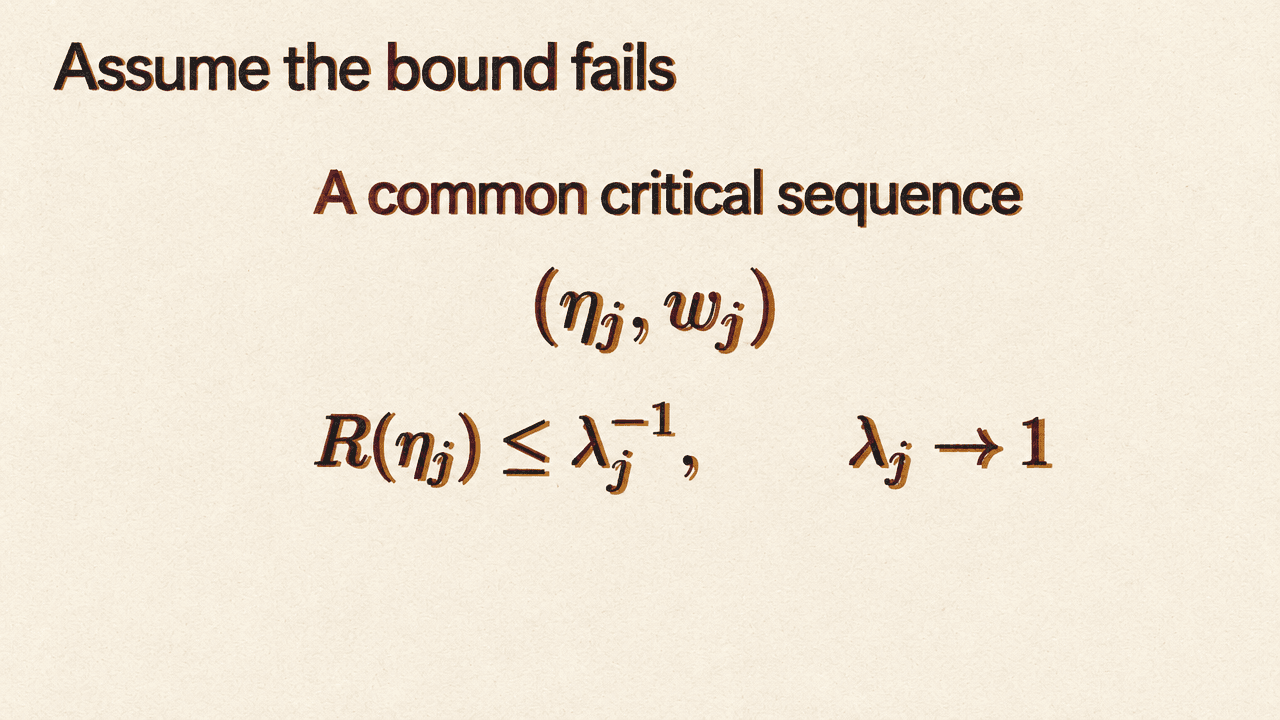
The proof’s central challenge is to get from controlled linear projections to a dimension-free entropy coefficient without relying on a dimension-free bound for the whole norm. The elementary norm estimate cannot do that: it carries a factor of n. Instead, the manuscript argues by contradiction, using the failure of the desired inequality to construct a sequence whose properties force incompatible bounds on an information integral.

Let 2R denote the best entropy coefficient. If the claimed inequality failed, the manuscript constructs hypothetical counterexamples with R fixed at one while their linear tail scales aⱼ tend to zero, and regularizes each distribution by adding Gaussian noise. There are two cases in the construction. If the logarithmic Sobolev constant exceeds the Poincaré constant, an entropy optimizer supplies a new law η and a vector field w. If the constants coincide, a first nonconstant eigenfunction supplies the field. Both routes lead to a critical sequence; η has a logarithmic Sobolev bound but need not itself be log-concave.

The key bridge is a rigid prediction curve for that sequence. Draw Y from η and observe Y after adding independent Gaussian noise of variance r. The manuscript proves that the squared norm of the conditional prediction of w(Y), divided by the original squared norm, tends to e⁻ʳ for each fixed r strictly between zero and one-quarter. This is not a general formula for Gaussian prediction. It is a constraint imposed by the hypothetical counterexamples. The manuscript uses that constraint to control fluctuations across scales, ultimately comparing the resulting matrix behavior with a scalar log-normal experiment.

The contradiction comes from integrating mutual information over observation scales T with weight dT/T². Under the assumed logarithmic Sobolev bounds, the manuscript obtains a universal limiting upper bound. Its fluctuation comparison gives a lower bound through the scalar log-normal experiment; when diffusion time and covariance cap grow together, that lower comparison becomes arbitrarily large. The construction therefore links the hypothetical failure of a dimension-free entropy coefficient to an information quantity that cannot remain both bounded and arbitrarily large.

The order of limits matters: first take the limit along the hypothetical counterexamples with time and cap fixed; only afterward choose those fixed parameters sufficiently large. The upper and lower bounds then conflict. This is the manuscript’s route around the dimension loss in the direct norm estimate—not a separate assertion that the distribution’s radius is dimension-free.