Schrödinger Waves Converge Pointwise at the Sobolev Endpoint in Dimensions Three and Higher

For the free Schrödinger equation, each frequency evolves by a rotation of its complex phase. Infinitely many frequencies can interfere at one spatial point, so convergence in an average, squared-error sense does not guarantee convergence almost everywhere. The mathematical question is whether the wave returns to its initial value pointwise for rough data, at the exact regularity threshold where earlier results cited in the paper establish convergence only above it.

That threshold is the Sobolev exponent $s_n=n/(2(n+1))$, where $n$ is the spatial dimension. In three dimensions, $s_3=3/8$. The result claims convergence for every complex-valued datum in this Sobolev space, in each fixed dimension $n\ge 3$, without radial symmetry, additional smoothness, or logarithmic strengthening. Counterexamples below the threshold do not settle the equality case. The planar endpoint is treated in a separate companion manuscript.

For rough data, the evolution is defined using Gaussian regularization: each Fourier coefficient is multiplied by $e^{(}-a|\xi {|}^2)$, with $a>0$. The order of limits matters. First remove the damping by taking $a\to 0$; then take time down to zero. For each datum, one spatial set of full measure works for every real time between zero and one. On that set, removing the damping is uniform in time; the approximation error is then driven to zero by improving the approximation. The resulting path is continuous down to time zero, and its limiting value is the datum’s Lebesgue value, defined through local spatial averages.^†

The endpoint difficulty appears when the datum is split into frequency bands of doubling size. Its Sobolev norm combines the weighted sizes of those bands through a square sum. But if each band is bounded separately at its worst time and those bounds are then added, the argument may demand an ordinary sum instead. A square-summable sequence need not be summable: the sequence $1/j$ has finite square sum but divergent ordinary sum. This illustrates the obstruction; it is not a counterexample to the wave estimate.

A fixed extra power of frequency would also demand more regularity. At the endpoint there is no spare regularity to spend, so the proof needs a bound with exactly the required frequency factor, not one weakened by an arbitrarily small loss.

The method for obtaining that bound is geometric. It decomposes waves into packets and controls where transverse families of packets can be large together. Fractal and transverse estimates supply a sparse gain; an induction studies concentration near polynomial walls; curvature tests and flattening reduce relevant pieces to affine plates, where a lower-dimensional frame estimate applies. The resulting short-time weak bound holds for some $p>2$ with precisely the endpoint frequency exponent. This is a roadmap through the packet geometry; the detailed geometric arguments and imported analytic ingredients are not reproduced here.

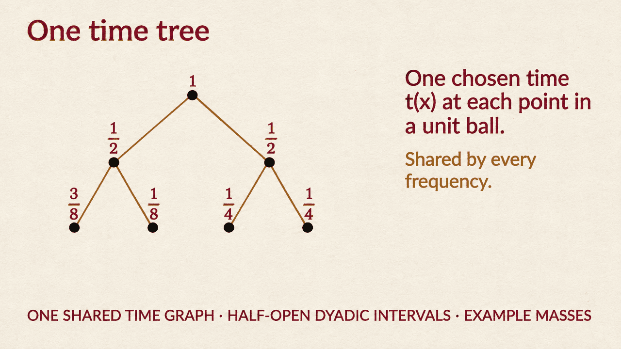
The next problem is to combine frequency estimates without losing the endpoint. The bookkeeping can be understood using one fixed unit ball in space. At each point, choose a measurable time in $[0,1)$, the same chosen time for every frequency. Repeatedly bisect the time interval, assigning boundary times to only one child. Each interval receives the measure of points whose chosen times lie in it, so a parent’s mass is the sum of its children’s masses. These are masses, not wave amplitudes or energies.

At each split, call the larger child’s mass $a$ and the smaller $b$. The short-time estimate gives an exponent $\alpha =3/2-1/p$. Since $p>2$, $\alpha >1$. That strict inequality means the parent’s mass raised to $\alpha$ exceeds the sum of the children’s powers by enough to pay for the smaller child.

For $b>0$, set $u=a/b\ge 1$. The relevant difference, divided by $b^{\alpha }$, is $(u+1{)}^{\alpha }-u^{\alpha }-1$. Its derivative is positive when $\alpha >1$, so its minimum for $u\ge 1$ occurs at $u=1$, where it equals $2^{\alpha }-2>0$. Thus each split charges at least $(2^{\alpha }-2)b^{\alpha }$ to the parent-minus-children difference. If $b=0$, the inequality is immediate.

Summing over a finite tree makes the internal terms cancel: every internal mass power appears once positively and once negatively. The total of the lighter-child charges is therefore bounded by the root’s mass to the power $\alpha$, divided by $2^{\alpha }-2$. The bound does not grow with tree depth. This accounting is used across frequency bands: at each fixed relative depth, different frequency indices correspond to distinct parents, so no parent is charged twice. Summable frequency weights then control the contributions from different relative depths.

The final step turns the local estimates into pointwise convergence. Smooth, compact-frequency approximations are chosen with summable Sobolev errors. Their evolutions converge uniformly in time outside one null set, and a uniform limit of continuous time paths remains continuous.

To connect that limit to Gaussian regularization, countably many error envelopes are used, each defined by taking a supremum over all times. Gaussian averaging recovers each envelope at its Lebesgue points. First the damping is removed; then the approximation is improved, driving the error to zero. Taking the time supremum inside the envelopes is crucial: it avoids intersecting an uncountable collection of time-dependent full-measure sets.

The stated result is that, for $n\ge 3$ and $f\in H^{(}n/(2(n+1)))(R^n)$, the Gaussian-defined evolution returns to the datum’s Lebesgue value as time approaches zero, for every real time in the interval on one full-measure spatial set. That set may depend on the datum. The tree inequality explains one part of the endpoint summation; the packet geometry and its analytic inputs remain essential to the global proof.