A Sharp Three-Dimensional Kakeya Bound Tracks Sparse Tube Density
An OpenAI manuscript claims a sharp three-dimensional Kakeya maximal estimate, allowing a δ⁻ε loss as tubes become thinner. Its central claim is density-sensitive: the bound must hold even when only a sparse subset of each tube is retained, with the resulting union estimate weakening cubically in the retained fraction. The manuscript’s proof argues that near-extremal tube families must recur in a constrained geometric pattern across scales, then uses projection and information estimates to rule out the configurations that would violate the bound.
The density of the shading is part of the theorem
The September 2026 OpenAI manuscript claims a sharp three-dimensional Kakeya maximal estimate. Its central issue is not simply how thin tubes overlap, but how much of each tube is retained. The claimed bound is intended to remain meaningful even when the shaded portions are sparse. The claim appears in the manuscript’s Theorem 1.1.†
Take a cylinder of length 1 and radius δ, whose volume is πδ². Regard a function f as brightness distributed through space. For each direction ω, slide the cylinder to every possible center and take the largest average of |f| over it. This gives the maximal function Kδf(ω). The manuscript claims that its L³ norm over directions is bounded by the L³ norm of f in space, up to a factor Cε δ⁻ε:
||Kδf||L³(S²) ≤ Cε δ⁻ε ||f||L³(ℝ³).
For every positive ε, the constant may depend on ε, but not on δ or f. This is not a scale-independent bound: it permits a small loss as the tubes become thinner.
The density-sensitive version makes the role of sparsity explicit. Let each tube T contain a selected subset Y(T) occupying at least a fraction λ of its volume. For tubes in a fixed bounded region with δ-separated directions, the desired lower bound for the union of the selected subsets is a constant times δ^ε λ³ times the sum of the tube volumes. The cubic dependence matters: when λ is small, the bound weakens rapidly. A much larger power of λ would make the bound weaker still. Earlier set estimates are inputs to the manuscript’s argument, not substitutes for this conclusion, which must hold uniformly for every 0 < λ ≤ 1.
Equal density can conceal different behavior across scales
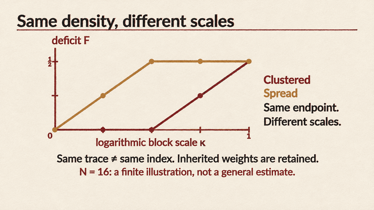
To handle sparse selections, the proof tracks which time bins along each tube are marked. A finite illustration divides a tube into 16 bins and marks four, so the density is 1/4. Two arrangements can have that same total density while behaving differently inside a block of four bins: one block may be full, while another contains only one mark. The illustration contrasts these patterns and plots their deficit profiles against logarithmic block scale. It is a finite example, not a general estimate.
The temporal deficit profile records missing branching at different block sizes. Its horizontal axis is logarithmic scale, not physical time. Total density determines the endpoint of the profile, but the curve across scales also matters when the configuration is rescaled. The bookkeeping retains each original tube index and its weight, even when distinct indices share the same geometric trace.
The proof’s structural reduction asks what a family approaching equality in the critical multiplicity bound would have to look like. The manuscript uses local mass bounds and multilinear Kakeya to force directions near a common plane on typical short blocks. Planar Furstenberg estimates and a plate-filling argument then reveal further structure. Restrictions and rescalings produce a stationary configuration: its normalized shape and deficit pattern recur across scales.
For that selected hypothetical near-extremizer, the canonical deficit profile is initially flat and then rises linearly. These claims do not describe every tube family. They constrain the special configuration that would witness failure of the desired estimate. The structural arguments are substantial and are not detailed here.
Two coordinate changes produce the product the proof needs
One local algebraic step shows how the geometric structure feeds into the later information argument. In a coordinate chart, a tube center line is an affine graph, Mᵢ(t) = bᵢ + t uᵢ, with two position coordinates and two slope coordinates. Choose a normal parameter ϑ and define sheared coordinates: X = Mᵢ(t)₁ + ϑMᵢ(t)₂, Y = Mᵢ(t)₂, U = uᵢ,₁ + ϑuᵢ,₂, and V = uᵢ,₂. These are sheared coordinates, not a rigid rotation.
Now change time by a. Position changes to (X + aU, Y + aV), while slope stays fixed. Then change the normal parameter by b. The new first position coordinate is X′ = X + aU + b(Y + aV), or, after expanding, X + aU + bY + abV. The mixed term abV follows from composing the two changes; it is not an approximation inserted into the argument. With the middle coordinates held fixed, it gives a projection involving X and V with product slope ab.
The information argument depends on both projections and dependence
The stationary packets require information in the four coordinates X, Y, U, and V. Conditional entropy tracks that information as cells are refined. But the changed coordinates are also projections of the original ones, so planar projection estimates constrain how quickly the information can grow. When the refinement speeds for the middle coordinates coincide, the proof needs an additional product-slope pinning argument.
A separate issue is dependence. The two events being compared share the same original tube index, so their random variables are not automatically independent. The paper compares their actual joint law, conditional on base data, with a conditional product law. Mutual information controls the discrepancy. Assuming independence outright would omit an essential part of the proof.
The final contradiction compares the information demanded by the stationary configuration with the limits imposed by the projection estimates. The manuscript’s case analysis treats distinct and tied refinement speeds, including boundary and zero-rate cases, and establishes h(p, 0) = 0 for parameters p > 2 arbitrarily close to 2. Here h is the extra resolution exponent. The displayed parameter relations clarify how this vanishing is used: choose p close enough to 2 that (p − 2)/3 < ε, then take κ = ε/2. The paper’s reductions transfer the discrete estimate through indicator functions to general L³ functions; the remaining small losses can then be absorbed into the prescribed ε, yielding the δ⁻ε factor in the maximal bound. This is the bridge from the case analysis to the claimed theorem, not a direct consequence of the equation h(p, 0) = 0 alone.
The claimed maximal estimate thus rests on more than tube overlap: the argument passes through recurring geometric structure and information constraints, including the dependence between events associated with the same tube index. The coordinate identity is a local algebraic check; it does not by itself verify the omitted global structural and analytic arguments. The explainer follows the pinned manuscript and is not an official OpenAI production or an independent certification of its proof.