Prime Predecessor Factors Converge to the Poisson–Dirichlet Law

For a prime p, factor p−1, take the logarithm of each prime-factor occurrence, and divide by log(p−1). The resulting pieces sum to one: logarithms turn the product into a sum. Keep repeated factors as separate pieces, then sort them from largest to smallest.

For example, 73−1 = 72 = 3·3·2·2·2. Each occurrence of 3 accounts for about 25.7% of log 72; each occurrence of 2 accounts for about 16.2%. The manuscript’s claim is that, as primes grow, the leading pieces of this ranked partition approach a universal random law.

That law can also be constructed by breaking a stick of length one. Make an independent uniform cut in the remaining stick at each step, keep the fragment cut off, and continue. The fragments are not produced in size order, so sort them afterward. Their ranked sequence has the Poisson–Dirichlet distribution with parameter one, or PD(1).

The manuscript identifies its main result as the Ford–Konyagin–Luca conjecture. Choose a prime uniformly from the primes between 3 and x. For any fixed number k of leading coordinates, the joint distribution of those normalized logarithmic factor sizes converges, as x grows, to the first k ranked pieces of the PD(1) stick-breaking partition.^†

The details of the sampling matter. Each prime receives equal weight; factor multiplicities count; and the normalization is by log(p−1). The result is not a claim that every individual prime has a typical-looking factorization. Nor does joint convergence say that the ranked pieces are independent.

The proof has two distinct jobs. Analytic estimates must establish a local law for factor occurrences in the interior of the possible size range. A probability argument must then turn that counting law into the full ranked limit, without losing mass near the boundary or in the small, undrawn pieces.

If a product D of selected distinct prime divisors divides p−1, then p must be congruent to 1 modulo D. As the selected factors grow, so does the modulus. To describe factor combinations whose logarithmic sizes together approach the full mass of one, the proof needs estimates that remain effective for large combinations.

The manuscript’s roadmap describes two new estimates. One uses small-prime-divisor marks and a memory expansion that retains dependencies between repeated prime factors. A second places marks on both sides and draws on operator theorems from a companion manuscript, along with new endpoint estimates. Pre-sieving and averaging away the marks then yield the interior factor statistics. The explainer omits these long analytic estimates; its probability argument depends on their output rather than replacing them.

A congruence condition is not a primality test: p congruent to 1 modulo D is necessary when D divides p−1, but does not establish that p is prime.

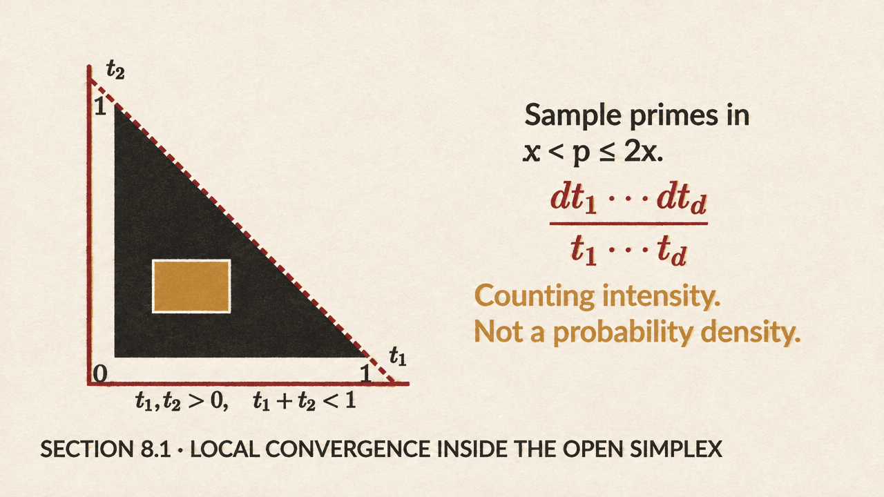
Temporarily sample primes in an interval x < p ≤ 2x, and treat each prime-factor occurrence as its own piece, with mass equal to its logarithmic size divided by log(p−1). For ordered selections of distinct occurrences with masses t₁ through t_d, the limiting interior counting intensity is the product of dtᵢ/tᵢ over the selected masses, where the masses are positive and their sum is less than one.

This intensity counts selections; it is not itself a probability density. The result initially applies away from zero and away from the boundary where the selected masses sum to one. Sorting at this stage would leave open the possibility that probability has escaped into those excluded regions.

The bridge is to sample pieces in proportion to their mass, not uniformly by occurrence. For the first draw, the selection probability contributes a factor t₁. Multiplying by the counting intensity cancels the 1/t₁, leaving dt₁: the first selected mass is uniform on the interval from zero to one.

After a first mass t₁ is removed, the remaining mass is 1−t₁. A second piece of mass t₂ is selected with probability proportional to t₂ divided by that remainder. Multiplying the two selection probabilities by the two-piece intensity cancels both mass factors and leaves dt₁dt₂ divided by 1−t₁. For fixed t₁, the second mass is uniform across the remaining interval. Expressed as a fraction of that remainder, it is a fresh uniform draw. The same cancellation at every step gives independent uniform relative cuts—the stick-breaking construction—even though the resulting fragment sizes are dependent.

The transformed density for the first two draws integrates to one over the triangle where t₁ and t₂ are positive and their sum is less than one. More generally, the proof uses the fact that the limiting size-biased draw law accounts for the full probability mass: interior regions can capture arbitrarily close to all of it. Because the original draw laws are probability measures, no additional limiting probability can remain at the boundary.

A second safeguard handles the pieces not yet drawn. After d size-biased draws, the expected undrawn mass is 2 to the power of −d. Sorting the drawn pieces approximates the ranked full partition; each ranked coordinate can differ from its full-partition counterpart by at most the mass left undrawn. Taking the prime-size limit first and then letting d grow makes that error vanish.

Finally, the proof transfers the result from primes in a doubling interval to all primes up to x, using a finite decomposition into intervals such as (x/2, x], (x/4, x/2], and so on, before letting the discarded fraction vanish. The analytic estimates supply the arithmetic counting law; size bias, boundary control, and sorting convert it into the stated joint PD(1) limit.