Meta Flow Maps Cut Reward-Alignment Costs With One-Step Posterior Sampling
Peter Potaptchik presents Meta Flow Maps as an amortized way to remove a costly inner loop in reward-aligning generative models: repeatedly simulating trajectories to estimate expected future reward from a noisy state. The method trains stochastic flow maps to produce differentiable, one-step samples from the clean-data posterior conditioned on any time and noisy state, enabling value-gradient estimates for inference-time steering and an off-policy objective for fine-tuning. In ImageNet experiments, Potaptchik argues, this lets a single-particle steered sampler outperform Best-of-1000 baselines across several rewards with far less compute.
The bottleneck is estimating future reward, not naming the reward
Peter Potaptchik frames Meta Flow Maps as a way to make reward alignment cheaper by replacing repeated trajectory simulation with one-step posterior sampling. The alignment target is a reward-tilted distribution,
where is the original data distribution and is a downstream reward. The reward can come from likelihoods in inverse problems or from black-box neural networks that score whether humans like an image or whether it follows a prompt.
There are two standard ways to use such a reward. In inference-time steering, the model weights stay fixed and the sampling dynamics are modified on the fly. In fine-tuning, the model parameters are updated so that the model permanently targets the reward-tilted distribution rather than the original data distribution. Both routes run into the same computational object: the value function, the expected future reward from the current noisy state.
The value function is
The distribution is the posterior distribution of clean data samples consistent with a noisy state at time . The optimal steering dynamics, in the presentation, are governed by a Doob ODE:
The first term, , is the original generative drift. The second term is the correction that points the trajectory toward states with higher expected terminal reward. Potaptchik describes the form by analogy to Doob’s h-transform for controlled SDEs, then conversion into a probability-flow ODE. The derivation details are not the emphasis; the consequence is. Reward alignment requires estimating many times during sampling or training.
The immediate obstacle is that is an expectation under a posterior distribution over clean data. A straightforward approach would repeatedly roll out trajectories from the current noisy state to generate possible clean endpoints, evaluate the reward on those endpoints, and backpropagate or otherwise estimate the value gradient. The claim is that this repeated posterior sampling is the expensive inner loop Meta Flow Maps are designed to remove.
Meta Flow Maps target clean-data posteriors, not just the data distribution
The construction starts from transport-based generative modeling. A prior distribution , usually a standard Gaussian, is transported to a data distribution . In the stochastic-interpolant notation Potaptchik uses, a prior sample and a data sample are connected by a linear path,
Flow matching defines a vector field by the conditional expected velocity,
If an ODE initialized from follows this drift, its marginal law at time matches , and at time one it samples from . The drift can be learned by regressing a neural network against the interpolant derivative.
The cost of using such an ODE is numerical integration: sampling requires many evaluations of the drift network. Flow maps and consistency models address that by learning solution operators directly. Instead of integrating
a flow map is trained so that, along an ODE trajectory,
Setting and gives a one-step jump from noise to data.
The generalization is to add context. A context-dependent flow map can target a family of distributions by taking a context as input. Class-conditional generation is the simple example: fixing the class index asks the map to transport Gaussian noise into the distribution of cats, dogs, hamburgers, or another class.
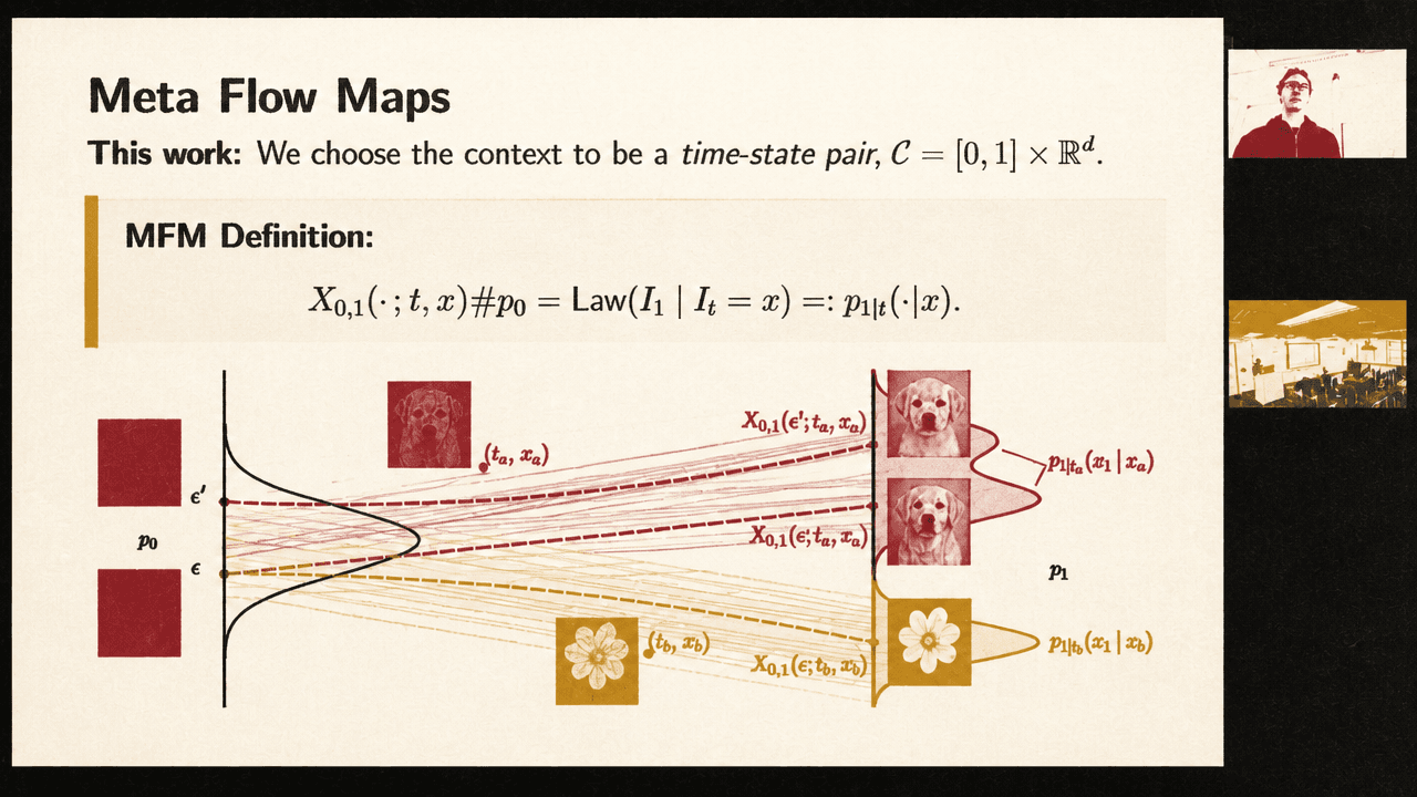
Meta Flow Maps choose a particular context: the pair , where is a time in and is a noisy state. For each such context, the target distribution is not the whole data distribution but the posterior clean-data distribution,
In words: given a noisy image state, generate independent plausible clean images that could have produced it. The ImageNet reconstruction slides show the posterior’s behavior. At larger noise levels, the posterior is broad: samples vary in color and details while remaining semantically related to the conditioning image. At smaller noise levels, the posterior concentrates: samples become much closer to one another and to the original clean image. In response to an audience question, Potaptchik clarifies that the shown example also includes class-index conditioning.
The distinction is central. A standard one-step flow map samples from . A Meta Flow Map samples from an infinite family of posterior distributions , indexed by all possible noisy states and times. The “meta” part is the amortization: the context selects which posterior-targeting flow map the network should act like.
The map must be stochastic and differentiable in the conditioning state
For steering, it is not enough to draw a single plausible reconstruction. The method needs a generative map
so that the value function can be written through a reparameterization,
The map must satisfy two conditions. First, for every , pushing forward the noise distribution must produce the correct posterior. Second, must be differentiable with respect to , because the steering term requires .
With those two properties, the gradient can be estimated by Monte Carlo:
In the Meta Flow Map instantiation, becomes , and the noise distribution is the prior . At each steering step, the sampler draws noise samples, maps them in one step into posterior clean samples conditioned on the current state, evaluates the reward, forms a log-sum-exp estimate of the value function, and backpropagates through the reward and the Meta Flow Map to obtain . That estimate is then plugged into the Doob ODE update.
The one-step nature matters because the estimator is used inside a loop. Backpropagating through a one-step posterior sampler is much cheaper than backpropagating through long inner rollouts. Potaptchik also notes that while the presentation primarily uses a gradient-based estimator for differentiable rewards, the work includes estimators for non-differentiable rewards using Stein’s identity, similar to tilt matching. In response to a question, he says those estimators do not rely on reward gradients.
Training reduces to flow-map training after conditioning on a context
Peter Potaptchik presents Meta Flow Maps as an extension of standard flow maps rather than a new generative-modeling paradigm. For each fixed context , define an auxiliary conditional ODE that transports the prior to the posterior :
The overbar notation separates this auxiliary ODE from the original unconditional generative ODE. The auxiliary drift can itself be defined by flow matching between the prior and the context-specific posterior. For a fixed context, there is a solution operator for that auxiliary ODE. The Meta Flow Map is a single neural network that represents this infinite collection of solution operators:
The two time variables play different roles. The context time identifies the posterior distribution being targeted. The flow-map times and are internal times for the auxiliary ODE that transports noise to that posterior. There is no ordering relation between and .
The parameterization mirrors ordinary flow maps:
The network is trained with a diagonal loss and a consistency loss. The diagonal loss anchors the instantaneous velocity to the true conditional drift . The consistency loss enforces the semi-group condition that makes the map a valid integrator:
This structure is deliberately agnostic to the specific consistency objective. Mean flows, shortcut losses, Eulerian losses, Lagrangian losses, and related consistency or flow-map objectives can be used, because the Meta Flow Map construction only requires that each conditional map behave like a valid flow map.
For training from data, Potaptchik uses coupled interpolants. Sample two independent prior points and , and one data point . Use and to form the query state,
then use the independent and the same to form the auxiliary path,
Conditioned on , the endpoint is distributed as the desired posterior , while remains an independent prior sample. This recreates the flow-matching setup for the conditional auxiliary ODE. The diagonal training objective regresses onto the auxiliary path velocity .
There is also a distillation route. If the prior is Gaussian and a pretrained unconditional drift is available, Potaptchik says a result from GLASS Flows gives the ground-truth conditional drift analytically as a combination of , the context state , and a reparameterized call to the original drift. The exact formula is not treated as essential; the important point is that the diagonal target can be evaluated without stochastic flow-matching variance. He describes this as a no-variance target: unlike ordinary flow matching, the minimizer can make the regression loss exactly zero against the conditional drift.
The ImageNet results test whether one-step posterior sampling is accurate enough to use
The main experiments discussed are on ImageNet at 256 by 256 resolution. The model is a latent diffusion transformer, SiT-XL/2, adapted to condition on the extra inputs required by the Meta Flow Map. The base model has 675 million parameters and the MFM version has 683 million, an increase of about 8 million parameters.
The training pipeline starts from a base flow matching model trained for about 800 epochs, followed by a DMF flow-map stage for about 80 additional epochs and an MFM stage for about 30 additional epochs. Potaptchik cautions that an MFM training step is more expensive than a flow-map training step, which is itself more expensive than a base flow-matching step, so epoch counts are not a direct compute comparison. His claim is narrower: adapting a pretrained flow map into a Meta Flow Map is much cheaper than the rest of the training process.
The MFM is not primarily intended as an unconditional sampler, but the authors still evaluate unconditional FID to check that it remains competitive after learning the much larger family of posterior maps. The reported ImageNet table gives the following FID scores for the stochastic few-step MFM model:
| Model | NFE | Parameters | FID ↓ |
|---|---|---|---|
| MFM-XL/2 | 1 | 683M | 3.72 |
| MFM-XL/2 | 2 | 683M | 2.40 |
| MFM-XL/2 | 4 | 683M | 1.97 |
There is no strong reason to use MFM for unconditional sampling if a base flow map is available; the point of this evaluation is to show that the model retains respectable unconditional sampling while also providing stochastic one-step posterior samples. The authoritative table result shown for MFM-XL/2 is FID 1.97 at four function evaluations.
The more relevant evaluation asks whether the model recovers the posterior distributions . The first posterior recovery metric noises real ImageNet images to a conditioning time , samples clean reconstructions from the posterior, and computes FID between those recovered samples and clean ImageNet images. The second metric estimates the value function using posterior samples and measures correlation with a high-fidelity, expensive SDE rollout treated as ground truth. The baseline is GLASS Flows rollouts using the teacher model.
MFM shows the largest gains in the small-NFE regime, especially at one or two function evaluations. On the posterior recovery plots, MFM with a small number of steps reaches roughly the level obtained by much longer GLASS rollouts, which Potaptchik characterizes as closer to 30 steps. That low-step regime matters because the value-gradient estimator is used repeatedly; long rollouts would make backpropagation through the estimator expensive.
The visual slide for posterior evaluation compares MFM and GLASS curves across conditioning times including , , , and . The MFM curves sit in the low-function-evaluation region where the steering estimator will actually operate, which is why Potaptchik treats one-step and two-step posterior fidelity as more important than asymptotic rollout quality.
One to 32 posterior samples are enough to beat Best-of-1000 in the tabby-cat steering setup
For inference-time steering, Peter Potaptchik focuses on a class-conditioned ODE targeting the ImageNet class “tabby cat.” The reward functions are ImageReward, PickScore, and HPSv2, all conditioned on the same prompt: “A high-quality, high-resolution photograph of a tabby cat.” He characterizes these reward models as scoring whether an image looks good to humans and aligns with the prompt.
| Steering element | Setup reported |
|---|---|
| Target class | Tabby cat |
| Prompt | A high-quality, high-resolution photograph of a tabby cat |
| Rewards | ImageReward, PickScore, HPSv2 |
| MFM-G posterior samples | 1 to 32 per step |
| Baselines shown | Best-of-N, DPS, and an MFM-Search variant |
| Best-of-N scale shown | Up to Best-of-1000 in Potaptchik’s comparison |
The gradient-based MFM steering method uses the Monte Carlo posterior estimator of . In the experiments Potaptchik discusses, the compute axis is controlled by the number of posterior samples used at each step. He says the evaluated range goes from one to 32 samples for this estimator. As the number of Monte Carlo samples increases, performance improves, which he describes as favorable inference-time scaling.
The central comparison is against Best-of-N: roll out many candidate samples and select the one with the highest reward. In the shown tabby-cat setup, Potaptchik says the MFM gradient estimator beats Best-of-1000 across the reward plots while using over 100 times less compute. He also points to an MFM search variant that does not use reward gradients and still outperforms Best-of-N in the shown experiments.
What you can see is that in many of these cases, in all these cases, our gradient estimator is beating Best-of-1000 and is doing so at over 100 times less compute.
The steering image grid makes the comparison concrete without relying only on reward curves. The first column contains base MFM samples of tabby cats. The second shows MFM-G using one Monte Carlo sample per step. The third shows MFM-G using 32 samples. Potaptchik presents the left-to-right progression as evidence that increasing the Monte Carlo budget strengthens steering and improves apparent sample quality without obviously collapsing into pure reward hacking.
A later question probes whether the improvement comes from a better value-gradient estimate or from smoothing non-smooth reward gradients by averaging. Potaptchik answers that smoothing may help, but argues it cannot be the whole explanation because the one-sample setting already beats Best-of-1000, where there is no averaging over multiple reward gradients. He also says behavior differs by reward, and agrees that ImageReward in particular showed interesting behavior worth investigating.
Fine-tuning uses the same posterior machinery but removes the self-normalized ratio
Peter Potaptchik does not spend the same amount of time on fine-tuning, but he gives the core construction and results. The goal is to distill the optimal steering drift into a student model so that the model is permanently aligned to the reward rather than steered at inference time.
The target drift includes a ratio:
Directly regressing against sampled estimates of this ratio would introduce the usual self-normalized estimator issue. The fine-tuning objective rearranges the optimality condition to multiply through by the denominator and put the condition under a single expectation:
In response to a question about how many Monte Carlo samples are used for fine-tuning, Potaptchik says the formulation does not have the same notion of a fixed sample count for estimating a ratio; training samples over , , and , essentially one sample at a time.
The ImageNet fine-tuning experiment trains across all classes using HPSv2 and the prompt template shown on the slide: “A high-quality, high-resolution photograph of a class.” The plots evaluate HPSv2, PickScore, and ImageReward during training. HPSv2 rises as expected, because it is the training reward, and PickScore and ImageReward also rise, suggesting the model is not merely exploiting HPSv2 in an isolated way.
The qualitative fine-tuning examples compare base samples with three separately trained reward strengths, labeled , , and . Increasing the reward weight increases the reward’s influence, with a middle regime producing nicer images and higher strengths eventually becoming oversaturated.
Two audience questions extend the fine-tuning idea. One asks whether, instead of learning only the instantaneous vector field , one could learn a flow map or even a Meta Flow Map for the fine-tuned dynamics. Potaptchik says yes: the presented objective helps with the instantaneous drift, and standard flow-map or self-distillation techniques could be layered on top to train a full flow map. Another asks whether one could directly learn a Meta Flow Map for the posterior distributions of the fine-tuned path. Potaptchik also says yes, though the presented work focuses on quick adaptation from an existing model to downstream rewards; he notes they are trying that direction.
The limits are statistical and representational, not only computational
The caveats in the discussion sharpen what Meta Flow Maps do and do not claim to solve. The first is reward variance. If has high variance under the relevant posterior, then estimating the value function may require many posterior samples. Potaptchik agrees with this concern. The method reduces the cost of each posterior draw by making it one-step and differentiable; it does not remove the Monte Carlo burden imposed by a high-variance reward. As one questioner summarizes, “there is no magic.”
The second caveat is diversity. Asked whether the method is closer to deterministic sampling and whether the authors studied sample diversity, Potaptchik says they did not look into diversity too much. He adds that the same steering can be done with SDEs, that ODEs were used for simplicity, and that their SDE results were similar. In theory, he says, the terminal distribution should be the same.
The third caveat is representation. An audience member notes that even simple velocity fields can have complex ODE solutions because the solution operator effectively composes the field with itself. That raises the question of why a flow map should be representable by a neural network of similar size to the one representing the underlying ODE. Potaptchik does not claim a general theorem. He says he is not an expert on that question, but believes there is work suggesting that Gaussian-to-data evolutions in these generative models have well-behaved properties that make flow-map training plausible. He agrees that for a generic ODE, learning the flow map could be hard; in this setting, it appears to work decently in practice.
These limitations leave the central claim narrower and more useful: Meta Flow Maps are not a general cure for difficult rewards or arbitrary dynamics. They are an amortized way to get the posterior samples that reward alignment already needs, cheaply enough to use inside steering and fine-tuning procedures.