Energy-Based Fine-Tuning Improves Accuracy Without RLVR’s Validation-Loss Penalty


Mujin Kwun and Carles Domingo-Enrich present energy-based fine-tuning as a post-training method that replaces next-token imitation or task-specific rewards with sequence-level feature matching. Their argument is that supervised fine-tuning remains efficient but is trained under teacher forcing, while RL with verifiable rewards can improve accuracy without preserving the target completion distribution. EBFT instead samples model rollouts, compares their frozen-model feature embeddings with reference completions, and uses that signal for policy-gradient updates; in the reported coding and translation experiments, it matched or exceeded RLVR accuracy while producing lower validation cross-entropy than both RLVR and SFT.
The post-training gap is sequence-level calibration
Mujin Kwun framed the work as a post-training problem: given a capable pretrained base model, such as Qwen, and a curated dataset for a downstream task, how should the model be adapted so that it preserves the benefits of pretraining while improving on the task?


The standard answer is supervised fine-tuning. SFT conditions on ground-truth prefixes and learns to predict the next token. That gives dense, stable, parallelizable supervision, and Kwun described it as a method that has worked well enough to become the default. Its limitation, in his account, is the train-inference mismatch. During training, the model repeatedly sees correct prefixes. During inference, it conditions on its own previous outputs. A small error in the next-token distribution can compound with generation length, producing miscalibrated outputs and a sequence-level distribution shift between model rollouts and ground-truth completions.
RL fine-tuning with verifiable rewards appears to address that mismatch because it operates on full rollouts and optimizes a sequence-level scalar reward. Kwun pointed to DeepSeek-R1-Zero’s math results as an example of correctness-based rewards improving downstream accuracy. But he argued that RLVR is not a general solution for two reasons. It requires a reliable reward signal or verifier for each task, and even when it improves task accuracy, it does not guarantee distributional calibration: it can optimize a scalar outcome while moving the model’s completion distribution away from the target distribution.
The proposed alternative is to match model completions to ground-truth completions in a feature space rather than at the token level or through a task-specific scalar reward. The objective asks whether the model’s rollout distribution has the same sequence-level feature statistics as the ground-truth distribution.
You take your model's rollout and you embed this rollout in this feature space, and you embed the corresponding ground truth in the same feature space. And you kind of just want to align these by minimizing the square loss.
The ideal feature-matching loss is:
Here is the context, is a ground-truth completion, is a model completion, and maps the context-completion sequence into a feature vector. Kwun emphasized that, under a rich enough feature map, this feature-matching loss is a strictly proper scoring rule: its unique minimizer is the ground-truth distribution.
That property distinguishes the proposal from both SFT and scalar-reward RL. SFT optimizes local next-token prediction under teacher forcing. RLVR optimizes a sequence-level scalar outcome. Feature matching targets sequence-level distributional statistics, and in the idealized case is minimized only by matching the ground-truth completion distribution.
The practical problem is that the ideal loss contains an expectation over the ground-truth completion distribution for a context, which is not available in ordinary datasets. The method therefore uses conditional feature matching, replacing the inaccessible conditional expectation with the observed ground-truth completion.
The derivation states that the conditional feature-matching loss and the ideal feature-matching loss differ by the expected variance of ground-truth features given the context, a term independent of . That means their gradients with respect to the model parameters are the same. The benefit of the conditional version is that the loss and its gradient can be estimated from ordinary context-completion pairs.
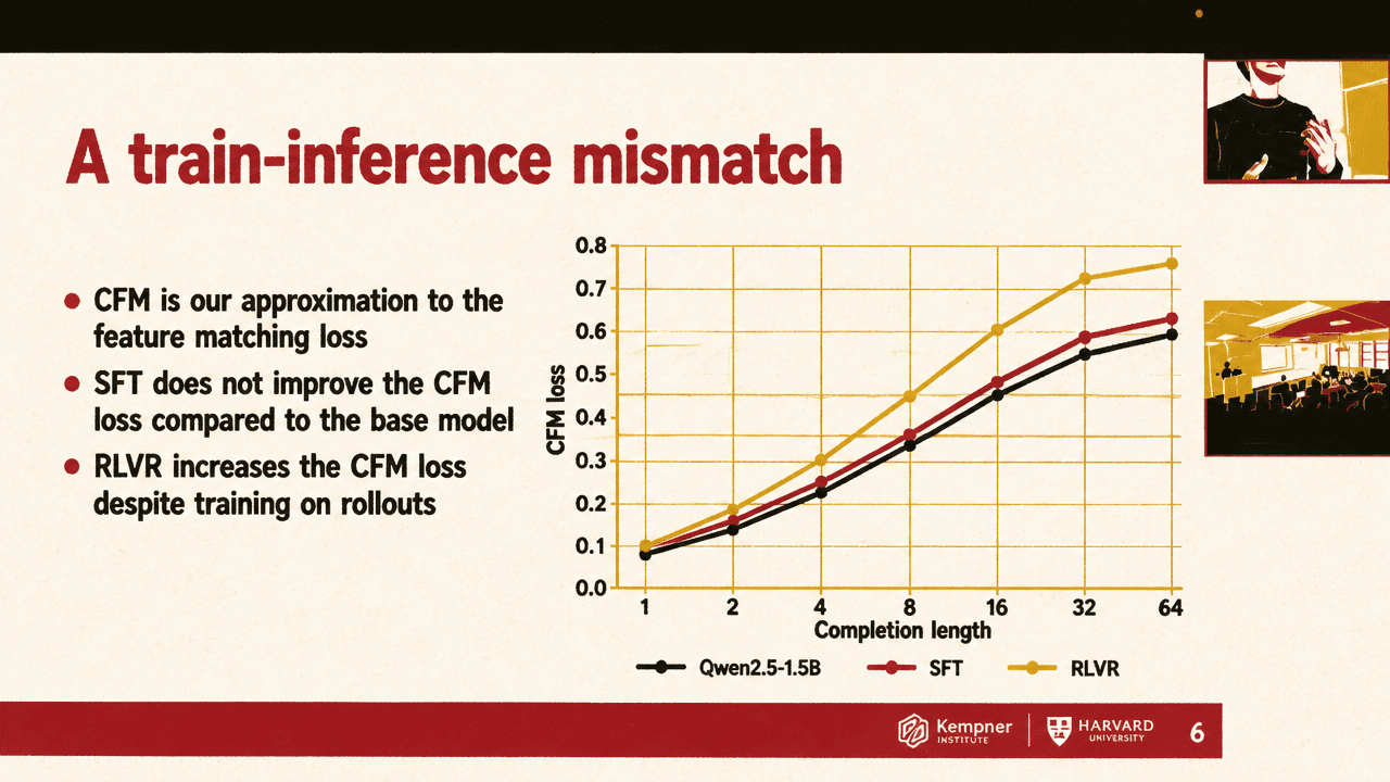
This also explains the behavior of the calibration plots. As completions get longer, the ground-truth distribution has more possible rollouts, so the variance term grows. With the ideal feature-matching objective, a well-calibrated model would have loss roughly constant across generation length. With the conditional approximation, some increase is expected because only a limited number of rollouts can be sampled. The empirical goal is therefore a lower curve that stays comparatively flat across lengths, not merely a low value at one rollout length.
Feature matching becomes a policy-gradient update
Operationally, EBFT trains with a policy-gradient update driven by feature vectors. For a context-completion pair, the model samples multiple on-policy completions. A frozen feature network embeds both the sampled completions and the reference completion. Rewards are computed from those embeddings, and the model is updated with an RLOO-style policy-gradient step.
The reward for a sampled completion has two terms:
The first term is an alignment term: it rewards completions whose features align with the ground-truth completion’s features. The second is a diversity term: it subtracts the average feature inner product between one sampled completion and the other completions from the same prompt. High-reward completions are therefore close to the ground truth in feature space while remaining diverse relative to the other sampled completions.
The reward is not introduced as a heuristic verifier. It comes from rewriting the gradient of the conditional feature-matching loss using the standard REINFORCE log-derivative trick. Since the ideal feature-matching loss and conditional feature-matching loss have the same gradient, the practical estimator is derived from that shared gradient while being computable from data.
The training loop used the context “The kids were excited because” and the ground-truth completion “it was the last day of school.” The generator sampled completions such as “summer break was starting,” “the circus was in town,” and “the weather was nice.” A frozen feature network embedded each generated sequence and the reference sequence. The method estimated conditional feature matching by comparing the mean sampled feature vector with the reference feature vector, then computed the alignment-plus-diversity reward for each completion and updated the generator.
The feature network is not a separately trained verifier in the experiments described. The authors construct features from activations in intermediate layers of a frozen copy of the actor model itself. Kwun described this as a design choice that yields rich embeddings, while noting that other choices may be possible.
The implementation also uses strided block-parallel rollouts. Instead of sampling one rollout at a time from one prefix, the method starts rollouts from multiple positions in a ground-truth sequence and generates them in parallel using interleaved generation and a custom attention mask. Kwun attributed this scheme to Quiet-STaR and described it as one of the more technically challenging parts of the work. In practice, he said, their rollout lengths are short.
The practical objective can also include an auxiliary cross-entropy term:
Kwun said the conditional feature-matching loss works on its own, but adding cross-entropy can help when the goal includes further improving cross-entropy values.
Cross-entropy and feature matching share a minimizer, not a landscape
In the simplest setting, if the feature map is one-hot and completions are length one, the feature-matching loss reduces to the squared distance between the model’s token probabilities and the ground-truth token probabilities:
Cross-entropy uses the same conditional distributions over the same token space, but applies a different penalty:
Kwun’s point was that the two objectives can have the same unique minimizer while producing different optimization behavior. In the one-hot, length-one feature-matching case, overshooting and undershooting ground-truth probability are penalized symmetrically. Cross-entropy penalizes undershooting ground-truth probability more heavily.
The distinction becomes more consequential once the objective moves from one-token probabilities to sequence-level feature statistics. SFT’s cross-entropy objective is local and teacher-forced. EBFT’s feature objective is computed over model rollouts. The training signal is still dense, because it uses feature vectors rather than a single binary success/failure outcome, but it is tied to the model’s own sampled completions.
That is the central positioning of EBFT: it aims to retain some distributional discipline associated with likelihood training while operating at rollout level and without requiring a task-specific verifier.
The empirical pattern is accuracy without the validation-loss blowup
The experiments tested two linked claims: whether EBFT improves conditional feature matching, and whether that improvement translates to downstream accuracy and validation cross-entropy.
In an early calibration plot on Qwen2.5-1.5B, the base model’s conditional feature-matching loss increased with completion length. SFT did not improve the conditional feature-matching loss relative to the base model at any generation length. RLVR made the conditional feature-matching loss worse, especially at longer completion lengths. EBFT, trained only on eight-token completions, improved the feature-matching loss across multiple completion lengths. Kwun highlighted that transfer across lengths as noteworthy.
The first downstream experiment used Qwen2.5-1.5B on a Q&A Python coding task from OpenCodeInstruct. SFT improved both downstream performance and validation cross-entropy relative to the base model. RLVR improved downstream task accuracy but greatly degraded validation cross-entropy. EBFT improved conditional feature matching and carried that into downstream results: the slide summary stated that EBFT beat SFT and exceeded or matched RLVR on downstream performance, while beating SFT on validation loss despite SFT directly optimizing cross-entropy.
The Q&A plots used coding metrics shown on the slides, including greedy and pass@16 views, alongside answer cross-entropy. The source visuals show plotted values rather than an exact reported table, so the following readings are approximate visual estimates and should be treated as secondary to the slide’s stated claims. In the pass@16 plot, EBFT ended around 0.74, RLVR around 0.72, and SFT around 0.64. On answer cross-entropy, EBFT ended near 0.26, SFT near 0.30, the base model near 0.28, and RLVR near 0.60.
| Method | Pass@16, approximate | CE loss, approximate | Pattern shown |
|---|---|---|---|
| Base Qwen2.5-1.5B | roughly 0.36–0.46 across plotted references | near 0.28 at the end | Base reference |
| SFT | near 0.64 | near 0.30 | Improves downstream and validation CE |
| RLVR | near 0.72 | near 0.60 | Improves downstream but degrades validation CE |
| EBFT | near 0.74 | near 0.26 | Matches or exceeds RLVR downstream while lowering CE |
Kwun presented the 40% figure as an internal note, not as a public benchmark table.
The same qualitative pattern appeared in translation. The model was Qwen2.5-1.5B trained on ALMA and evaluated with COMET on translation benchmarks including WMT22 and MTNT. SFT improved task performance and validation cross-entropy. RLVR, trained with a COMET reward on model generations and ground-truth data, again improved or matched downstream performance while increasing validation cross-entropy. EBFT optimized the conditional feature-matching loss, achieved better validation cross-entropy than both SFT and RLVR, and on downstream performance beat or matched RLVR.
For unstructured code, the point was different: RLVR is not naturally available because the dataset is not question-answer code with a straightforward verifier. Kwun described this as a setting where SFT would typically be the only obvious solution. The authors trained Qwen2.5-1.5B on SwallowCode and evaluated on HumanEval, MBPP, and MultiPL-E. EBFT matched SFT on validation cross-entropy while improving downstream metrics. A warm-started version of EBFT, initialized from an SFT checkpoint, further improved validation loss and conditional feature-matching loss while maintaining strong downstream accuracy.
| Method | Val CE | CFM | Greedy | Pass@1 | Pass@4 | Pass@16 |
|---|---|---|---|---|---|---|
| Base | 0.631 | 0.369 | 0.473 | 0.419 | 0.596 | 0.702 |
| SFT | 0.501 | 0.321 | 0.504 | 0.467 | 0.644 | 0.747 |
| EBFT | 0.499 | 0.320 | 0.548 | 0.524 | 0.664 | 0.769 |
| EBFT (warm-start) | 0.481 | 0.312 | 0.536 | 0.514 | 0.659 | 0.769 |
This table is directly visible in the source slide on “Beyond Verifiable Rewards.” The slide’s summary bullets state that EBFT achieved better downstream performance across the listed metrics and tasks, matched SFT on validation loss, and that warm-starting EBFT from an SFT checkpoint further improved validation loss and conditional feature-matching loss.
The scaling experiments tested Qwen2.5 models at 1.5B, 3B, and 7B parameters on structured Q&A coding data. For each trained model, the feature network was a frozen copy of the same-size actor. Kwun said the gains in validation cross-entropy, downstream performance, and feature-matching loss carried over across the tested model sizes, with no signs of diminishing returns in those experiments.
The feature map is the method’s main degree of freedom
The choice of feature map is central to EBFT. Mujin Kwun said the authors tested randomly initialized critics, mean pooling over token positions, and larger feature networks to understand whether the gains came from any high-dimensional representation or from useful semantic features.
Random weights still worked to some extent, but produced the worst performance among the tested feature configurations. The conclusion was not that random features are useless. Rather, even a high-dimensional random projection can give the method something to optimize, while trained or meaningful features perform better. Mean pooling over token positions and naively using a larger feature network did not provide much additional boost. In particular, using a larger Qwen2.5-7B feature network for a smaller model did not automatically improve results.
Kwun cautioned against overreading that result. In response to a question about whether crossing model families might produce more useful feature diversity than scaling within the same family, he said that could “definitely be true.” The team believes feature maps can be improved, and he mentioned internal experiments where training the critic seemed to help.
Carles Domingo-Enrich added a practical caveat: tokenization matters when using other models as feature networks. When the authors used models with different tokenizers, the setup did worse, but did not fail completely. In the question exchange, he said they were not detokenizing and retokenizing into the other model’s token space for that experiment. His interpretation was that if the feature representation is high-dimensional enough, the method can still do something, but better features should yield better performance.


The future-work version of this question is whether the features can be learned concurrently during training. Enrich said the group had explored candidates and wanted to determine whether learned features could produce meaningful and consistent gains. The tradeoff is non-stationarity: if the feature map changes during training, the target being optimized also changes, adding cost and complexity.
Self-likelihood is not the same as matching the target distribution
EBFT was positioned against other rollout-based approaches that do not require a straightforward verifier. Kwun’s critique was not that these methods are useless, but that their failure modes differ from the problem EBFT is designed to address.
Trained verifiers can be noisy and require careful training. Rubric-based and LLM-as-judge approaches can be useful, but they require careful engineering and may be hackable. The slides showed public posts about reward hacking and variability in LLM judging, including examples of agents taking shortcuts rather than solving tasks and discrepancies between reported and replicated judge scores. A longer post shown from Andrej Karpathy criticized RLHF-style training as weak on credit assignment because sequence-level rewards are assigned to full trajectories without search or intermediate value estimation.
Kwun also addressed verifier-free methods that reward generations based on self-likelihood. He said these methods can improve performance in many cases, but argued that optimizing self-likelihood does not have the same convergence property as feature matching: it does not, by itself, drive the model toward the ground-truth distribution. The authors ran a small experiment resembling EBFT but replacing feature-map rewards with rewards based on the model’s own perplexity on its own generations. Kwun said that degraded performance across the board.
That critique connects back to the calibration objective. If the target is not “make the model like its own outputs more,” but “make the model’s rollout distribution match ground-truth sequence-level statistics,” then self-likelihood is the wrong statistic. EBFT’s reward is not a model confidence score; it is a gradient estimator for feature-moment matching.
The output examples illustrated qualitative failures behind the metrics. In an English-to-French MTNT example, the source sentence was “Till Tigers will take revenge on those who have done wrong to them.” The SFT model repeated the English source rather than translating. The RLVR model produced a Portuguese-labeled Portuguese translation. EBFT produced a French translation: “Les tigres prendront leur revanche sur ceux qui leur ont fait du tort.”
The coding example was less cleanly aligned between the spoken description and the visible slide. Kwun said EBFT solved the task correctly, the base model returned an incorrect solution, and the RLVR model called functions that did not exist in the code context. The slide, however, labeled the RLVR output as “success, missing context,” while labeling the SFT output as incorrect and showing an EBFT success. The safe reading is that the example was used to contrast EBFT’s successful completion with baseline outputs that either failed or lacked the needed context, rather than as a fully specified benchmark result.
The task boundary was explicit. Kwun said RLVR works well for short-horizon problems that can be verified quickly and reliably, where scalar rewards capture the desired outcome: math, code, and tool use were the examples. But for long-horizon agentic tasks, scalar rewards can be too sparse; for subjective or non-verifiable tasks, there may be no ground-truth answer or reward function; and in niche, expert, data-sparse domains, there may be few high-quality demonstrations and no automatic evaluator. EBFT is positioned for that gap.
The energy-based view is an exponential tilt of a reference model
The name “energy-based fine-tuning” comes from a theoretical interpretation introduced by Carles Domingo-Enrich. Enrich considered a KL-regularized feature-matching problem: the optimized completion distribution is trained to match target feature statistics while remaining close, in KL, to a reference distribution , which may be another pretrained model or the starting model. The theoretical point of this KL-regularized view is that the solution has an explicit form.
That solution is an exponential tilt of the reference distribution:
Here is a maximum-likelihood vector inside a norm-bounded ball, with the ball size depending on the KL regularization parameter. Enrich’s interpretation was that this is the maximum-likelihood energy function for an energy-based model whose energy class is linear in the chosen features:
The method does not explicitly train an energy function. Under this view, the KL-regularized feature-matching solution corresponds to reweighting, or tilting, a reference distribution according to feature-based energies. Even without explicit KL regularization, Enrich suggested that the practical method can be thought of as related to the large- regime.
He then connected this to calibration. Suppose the goal is to match a target statistic,
while staying close to a reference distribution in KL. The optimal distribution again has an exponential-tilt form:
Enrich said Braverman et al. used this kind of framework to correct entropy drift in language model generations, choosing . That statistic is one-dimensional and tied to model log probability. EBFT instead chooses , creating high-dimensional moment constraints in a semantically rich feature space. This is also why the calibration view connects to the self-likelihood ablation: matching a one-dimensional likelihood statistic is different from matching high-dimensional semantic feature moments.
Whitening ties feature matching back to sequence-level divergence
All of the curves shown in the work used whitened features. Carles Domingo-Enrich explained the motivation: raw feature maps can have correlated or anisotropic directions, allowing some dimensions to dominate the feature-matching loss.
For each context and set of sampled completions, the method estimates a second-moment matrix:
It then defines whitened features using the Moore-Penrose pseudoinverse:
If the true second-moment matrix were available and used instead of the sample-based pseudoinverse estimate, Enrich said the whitened feature-matching loss would be a relaxation of the divergence between and , averaged over contexts. Since divergence is close to KL when two distributions are very close, the whitening view ties the method back to likelihood-style distribution matching, but at sequence level rather than next-token level.
He was explicit about the caveats. The method uses an approximate second-moment matrix from sampled completions, not the true matrix. The relationship is to , not exactly KL. And the pseudoinverse changes the reward balance: because it effectively projects ground-truth features into the subspace spanned by sampled completion features, it systematically reduces the norm of the whitened ground-truth feature. That weakens the alignment term and relatively strengthens diversity. To compensate, the authors normalize the whitened ground-truth and generated features only in the alignment term. Enrich called this “a bit of a hack,” but said it worked well and remains an active area of investigation.
The remaining questions are practical: cost, samples, and off-policy reuse
The authors’ future directions were mostly engineering questions. Enrich listed whitening variants, generation length, and the number of samples per prompt as important hyperparameters. Generation length is especially difficult because longer generations introduce more diversity and may resemble the ground-truth completion less often, making rollout comparison harder. The number of samples per prompt is related: the team wants to understand whether scaling samples helps in EBFT, even though standard RLVR does not usually scale that quantity beyond a certain point.
They are also studying robustness to data repeats in two senses: how many times to repeat ground-truth sequences, and how many times to reuse sampled rollouts during RL. In the Q&A, Kwun said they had internally tried a pipeline-style setup where generation and training are interleaved and samples may become off-policy. He said it seemed they could be “pretty off-policy” in that sense, and identified this as one of the main efficiency methods they want to explore.
Computational efficiency remains a central constraint. EBFT samples rollouts, extracts features, computes rewards, and applies a policy-gradient update. That is more involved than standard SFT. Enrich said the goal is to make the algorithm as fast as possible and competitive with SFT computationally. The team has already improved substantially over an earlier unoptimized version and believes a reasonable tradeoff is possible.
A final question asked whether the comparisons included the common pipeline of SFT followed by RL, rather than comparing EBFT only to SFT or RLVR separately. Kwun said they did run those experiments and that the ablations are in the paper. He summarized the result as EBFT still outperforming in validation cross-entropy and matching or exceeding downstream accuracy.