Self-Consistent Interpolants Learn Clean Priors From Corrupted Data
Jiequn Han’s talk argues that transport-based generative models should be treated not only as tools for sampling clean data distributions, but as machinery for recovering and adapting those distributions when the usual clean training set is absent. His main proposal, Self-Consistent Stochastic Interpolants, learns a clean prior from corrupted observations by iterating a transport map until the learned distribution, passed through a trusted forward simulator, reproduces the observed data. Han presents the method as a black-box alternative to EM-style inverse generative modeling, with the caveat that simulator mismatch remains a central unresolved risk.
The central problem is a clean prior without clean data
Jiequn Han framed measure-transport generative models as dynamical systems: learn an ODE or SDE that moves samples from an easy base measure into a target data distribution. In the standard formulation, samples are available from an unknown clean distribution , and the model learns an approximation that is both close to and easy to sample. Score-based diffusion, flow matching, rectified flows, and stochastic interpolants all fit this transport view.
The technical attraction is the continuous-time formulation. It connects particle dynamics, written as SDEs, to density evolution, written as PDEs such as Fokker–Planck equations. In score-based diffusion, a forward process adds noise to clean data; a reverse SDE is constructed so that its intermediate marginal densities match the forward process in reverse. The key learned object is the score, the gradient of the log density at intermediate time. Under simple forward processes such as Ornstein–Uhlenbeck or heat semigroups, Han noted, Tweedie’s formula identifies that score with a denoising oracle: a conditional expectation of the clean variable given a noisy observation. Since conditional expectations can be trained by regression, clean datasets become the practical basis for learning the score.
That assumption is precisely what fails in many scientific settings Han highlighted. Cryo-EM, medical imaging, particle physics, astronomy, and related inverse problems often produce abundant measurements but few or no clean samples. The data are blurred, projected, compressed, noisy, masked, or otherwise transformed by an instrument or simulator. The usual posterior-sampling framing—start with a pretrained clean prior, then recover a clean sample from a corrupted observation—does not apply if no clean prior can be pretrained.
Very often we may only have access to a lot corrupted data, but we do not have any access to the clean data.
Han’s inverse generative modeling problem is distributional. Given many samples from an observation distribution and black-box access to a stochastic forward simulator , the goal is to learn a generative model for the unobserved clean distribution . If induces a conditional distribution , it defines an operator mapping clean distributions to observation distributions. The goal is to solve the distribution-level equation .
Han described this as a linear equation over a density space. That does not make it easy. Once the data dimension is more than a few, directly solving the equation at the density level is not realistic. The alternative he presented is to solve the inverse problem at the distribution level with transport-based generative modeling.
The fixed-point equation also carries a practical condition. In the Q&A, when asked how the method handles mismatch between simulator noise and real-world noise, Han said the current work assumes a perfect simulator: in the infinite-sample case, there is a ground-truth model whose forward observations match the data. For model misspecification, he suggested a larger inverse problem may be needed. If the forward model has unknown parameters, one could jointly infer the clean data distribution and those parameters, with uncertainty quantification over the parameter side. But robustness to simulator mismatch remains, in Han’s account, an open and important question in the current pipeline.
Self-consistency turns missing clean samples into a fixed-point equation
Self-Consistent Stochastic Interpolants, or SCSI, were introduced as the main response to the no-clean-data setting. The method was developed with Chirag Modi, Eric Vanden-Eijnden, and Joan Bruna. Its starting point is the ordinary stochastic interpolant construction in the easier case where both clean and observation samples are available.
If one can sample from both and , one can draw a coupling , sample Gaussian noise , and define an interpolant as a linear combination of the clean endpoint, the observation endpoint, and the noise term. The coefficients are chosen so that has distribution and has distribution .
The drift and score-like term are conditional expectations:
Using these functions in reverse-time dynamics transports samples from at to at . The same notation covers ODE and SDE generation: setting the diffusion coefficient to zero gives an ODE, while nonzero gives an SDE. Training again resembles score matching, because the unknown functions are conditional expectations and can be learned through regression objectives.
Inverse generative modeling removes the clean endpoint. Samples from at are unavailable. SCSI replaces them with a guess that is iteratively made self-consistent.
Given transport parameters , the reverse dynamics defines a backward transport map from observed samples to candidate clean samples. Pushing through that map induces a candidate clean distribution:
The consistency condition is that if this induced clean distribution is passed through the true forward corruption operator, it should reproduce the observed distribution:
This is the fixed point. Given current parameters , SCSI pushes an observation backward to obtain a candidate clean sample . It then applies the black-box simulator to that candidate clean sample to obtain a simulated observation . A new stochastic interpolant is built between those two endpoints:
The next parameters are trained with the usual stochastic-interpolant regression objectives on this constructed interpolant. The outer loop updates the fixed point; the inner loop performs ordinary stochastic-interpolant optimization.
Han emphasized that the implementation remains close to standard stochastic-interpolant training. The inner loop samples an -side point, generates a corresponding simulated -side point through the forward model, constructs , and applies SGD. The extra structure is the outer loop that refreshes the transport map. That simplicity, in Han’s account, is what makes the method scalable to high-dimensional datasets and compatible with standard generative-model training.
SCSI avoids the two demands that make EM brittle here
Han compared SCSI with expectation-maximization because both use an iterative guess-and-update structure. In a classical EM approach to inverse generative modeling, one maintains a current prior . The E step generates posterior samples by Bayes’ rule, proportional to likelihood times current prior, and the M step updates the prior using those samples.
SCSI has a similar high-level shape: constructing a new interpolant from the current transport resembles an E step, and minimizing the transport objectives resembles an M step. Han’s distinction was practical. EM requires access to the likelihood in order to write Bayes’ rule. It also requires reliable posterior sampling. The adaptation portion of the talk had already treated posterior sampling as difficult even when a clean prior exists. Han said this is why earlier EM-style work was limited to settings such as linear inverse problems, where posterior sampling is more reliable.
The benefits of our self-consistent stochastic interpolant is that we only require a black-box simulator, we don't need the likelihood form for this simulator.
That black-box formulation is meant to make SCSI applicable to nonlinear forward models, non-differentiable forward models, and non-Gaussian noise. It is not a claim that the simulator can be arbitrary or wrong. Han’s caveat about perfect simulators is therefore central: self-consistency can replace clean samples only if the forward process used in training is the right one to enforce.
The reported experiments ask whether corrupted observations alone recover useful clean structure
The empirical SCSI results were framed around whether a transport prior can be learned from corrupted observations alone. On AFHQ images, Han showed three corruption models: random masking, Gaussian blur with noise, and motion blur with noise. For each forward model, SCSI was trained separately on the corresponding corrupted dataset. The examples compared original clean images, corrupted images, SCSI restorations, and DPS restorations.
The comparison to DPS was important but asymmetric, as Han described it. DPS is a posterior-sampling method that assumes a pretrained generative model trained on clean data, so it uses more information than SCSI. Han’s point was that SCSI, without access to clean data, still restored the corrupted images well, while DPS sometimes showed artifacts.
| Forward model | SCSI | DPS | SI-Oracle |
|---|---|---|---|
| Random mask | 0.0051 | 0.0049 | 0.0044 |
| Gaussian blur | 0.015 | 0.025 | 0.011 |
| Motion blur | 0.011 | 0.012 | 0.003 |
The restoration table showed SCSI close to DPS and the oracle on random masking, lower error than DPS on Gaussian blur, and similar error to DPS on motion blur, while the oracle remained best on motion blur. Han summarized the slide as showing that SCSI can match or, in some cases, exceed restoration performance of models trained with clean data, depending on the corruption and comparison.
A second slide measured generation after training a generative model using restored samples. SCSI’s generated FID was reported as 5.38 at , compared with Ambient Diffusion at 11.70, EM Posterior at 5.88, and a clean-data baseline at 5.16.
| Method | ρ | FID ↓ |
|---|---|---|
| Ambient Diffusion | 0.20 | 11.70 |
| EM Posterior | 0.25 | 5.88 |
| SCSI (generated) | 0.25 | 5.38 |
| Baseline | 0.00 | 5.16 |
A JPEG compression experiment on CelebA tested a nonlinear and non-differentiable forward model. The forward model used JPEG quality factors, where lower quality means stronger compression. SCSI was trained on compressed data with quality factors uniformly sampled from 10 to 50, then tested on qualities including 70 and 90, outside that training range. Han said the learned transport model still produced good restorations.
The final example used one-dimensional quasar spectra from cosmology rather than two-dimensional images. Two forward models were considered: high spectral resolution with low signal-to-noise ratio, and low spectral resolution with high signal-to-noise ratio. Han said SCSI performed much better than a standard method that applies an inverse solver to each individual sample.
The methodological claim was that many scientific inverse problems are usually solved sample by sample, while SCSI attacks a distribution-level inverse problem by using all available data jointly. Han acknowledged that this is harder, but argued that large-scale generative modeling makes this distribution-level route possible.
A Gaussian channel gives a tractable convergence case
For theory, Han presented an additive white Gaussian noise setting where the fixed-point iteration can be analyzed explicitly. The clean prior is Gaussian, . The forward model adds standard Gaussian noise, . The initialization is another Gaussian, . The interpolant is linear:
with constant diffusion .
In this case, every fixed-point iterate remains Gaussian, so the mean and covariance can be tracked across iterations. The proposition on the slide gave linear convergence rates. If and , then both covariance and mean errors contract geometrically, with a contraction factor involving .
Han drew several consequences. The ODE case optimizes the displayed upper bound, matching his observation that ODE versions sometimes converged fastest in imaging experiments. EM corresponds to in this setting. In the low-SNR regime where , SCSI with converges faster than EM; the slide contrasted rates of and . Han also said the paper proves convergence in both and KL under condition-number assumptions, which are abstract but verifiable in this Gaussian linear case.
Adaptation explains why the clean prior is worth recovering
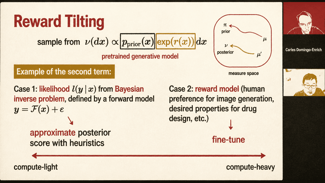
The no-clean-data problem matters because a good clean prior is useful beyond unconditional generation. Before introducing SCSI, Han described several ways to adapt a pretrained measure-transport model to related distributions.
A pretrained model defines a prior density . Adaptation asks for samples from a related density rather than from itself. One example is annealing:
Changing changes the effective temperature: in Han’s schematic, one direction scattered the distribution more broadly, while the other concentrated it into lower-temperature regions.
A second and more common form is reward tilting:
Bayesian inverse problems provide one interpretation. A pretrained generative model supplies the prior, an observation is related to clean data through , and the posterior is proportional to prior times likelihood. In that case, the reward term corresponds to the likelihood. A learned reward model supplies another interpretation: human preference in image generation, desired properties in drug design, or desired structure properties in protein generation.
Han placed existing methods on a compute spectrum. At the light end, methods approximate or modify reverse dynamics with heuristic posterior-score terms. These can be cheap and effective, but their approximation error is not controlled: one may not know what distribution is actually being sampled. At the heavy end, methods fine-tune model weights, especially when the reward model is complicated.
One alternative, developed with Joan Bruna, applies to quadratic, well-conditioned rewards, as in some linear inverse problems. The method changes the initial distribution rather than the learned reverse dynamics. If the original reverse SDE transports a Gaussian initial distribution into the prior, then for a suitable posterior target one can start the same reverse SDE at a different “boosted” initial distribution at a chosen time . In Han’s Gaussian-mixture illustration, the target posterior had shifted modes and weights; the boosted initial distribution was not Gaussian, but was closer to log-concave and therefore easier to sample. The theorem in that work characterizes when this boosted distribution becomes log-concave, enabling MCMC sampling with guarantees.
DriftLite, developed with Stanford collaborators, was presented as another adaptation route: make Sequential Monte Carlo more useful for diffusion-model adaptation by controlling the drift. Pure guidance defines a target path such as
and then modifies the reverse drift using terms such as the prior score and reward gradient. Han’s answer to whether that drift exactly tracks the intended density path was explicit: no. Fokker–Planck analysis shows that an additional reweighting potential is needed. SMC can carry that correction through particle weights, but finite-particle systems suffer weight degeneracy; the asymptotic convergence can be hidden by variance.
DriftLite uses the degree of freedom between particle motion and particle weights. Instead of letting all the correction appear in weights, it adds a lightweight control to the drift so the weights are less volatile. The full optimal-control characterization leads to a Poisson equation, but the practical method restricts the control to a linear combination of a few guidance-like basis functions: the prior score, the prior drift, and the reward gradient. In the three-basis version shown, the variance-controlling objective reduces to a small least-squares problem and a linear system estimated from particles.
| Method | Reported MMD |
|---|---|
| Pure guidance | 0.848 |
| Guidance + SMC | 0.249 |
| VCG-SMC | 0.018 |
The reported result was that ordinary SMC correction improved on pure guidance, and variance-controlling guidance with SMC improved further. Han also showed particle-scaling plots where pure guidance and ordinary guidance-plus-SMC did not visibly improve even with particle counts as large as , while the variance-controlled methods improved as particle count increased.
A third adaptation route changes the conditioning embedding rather than the generated state. In protein diffusion models, the conditioning vector may encode sequence information; in image generation, an analogous role is played by the text prompt. Han said inference-time embedding optimization shifts the prior toward structures that are physically plausible and consistent with experimental measurements. He did not detail the algorithm, but said it produced better reconstruction quality than a fixed-prior DPS-style baseline in the protein task, was more robust across hyperparameters, and allowed faster inference with fewer diffusion steps.
The questions narrowed the assumptions and practical costs
A question relayed by Carles Domingo-Enrich asked whether, for cryo-EM, the embedding-optimization reward should be defined directly on 2D particle images rather than on a reconstructed 3D map, and whether a sequence-derived embedding is still a useful manifold for steering toward conformations consistent with raw image data.
Han answered that the current experimental setting uses a reconstructed 3D map to define the reward, making it possible to compare a current structure directly against that map. With only 2D measurements, the reward is harder to define because it must handle alignment between 2D projections and original 3D conformations, and may even be non-differentiable. He said this is an open question his collaborators are working on: whether useful rewards can be designed from 2D images for steering either coordinates or embeddings.
On whether sequence-based embeddings remain useful, Han said he thought so, because the object is still protein conformation. MSA-type information may be limited, but he viewed it as a useful starting point. He also suggested a broader pretraining question: whether embedding modules can be designed so that post-training steering becomes easier and more flexible.
Carles also asked how many outer-loop iterations SCSI used. Han answered that it depends on the number of inner-loop optimization steps. Conceptually, the inner loop can be described as finding the minimizer for the interpolant, but doing that fully in early stages would be inefficient. In implementation, he said, the inner loop can be as small as 10 or 20 steps before the outer loop is refreshed. If the inner loop is set to one, the method resembles a stochastic-gradient-style update. Han said modest inner-loop counts larger than one gave more efficient performance.
On dataset size, Carles asked whether SCSI needs substantial data because it is effectively pretraining a flow model at every iteration. Han agreed that more data or more training is needed than in standard clean-data training, especially for more singular or ill-posed forward models. But in their experiments he characterized the gap as moderate, perhaps around a factor of 10, and noted that they used a dataset at the scale of CIFAR-10.
Asked whether SCSI could be combined with an imperfect pretrained model, Han said yes. Their implementation tested the extreme case of random initialization, with no prior knowledge. If a low-quality generative model or low-quality images are available, they can be used to pretrain an initial guess before applying the fixed-point iteration. Han described this as simply a better initialization, and likely the realistic route in many applications.
A final question returned to DriftLite. For a conditioned model, such as a text-conditioned generator, should the optimal coefficients be set separately for each conditioning or shared? Han said a common coefficient would be the easiest useful version, because it would allow inference with few particles. One possible route would be to apply the technique during an intermediate training phase across many text prompts and particles, optimize coefficients, and then use a common set at inference time. The experiments he presented were unconditional, but he said they observed shared coefficient patterns. Near clean data, guidance is already good; the main benefit is finding coefficients that help earlier in the trajectory. He expected the overall trend could be shared across instances.