Cross-Entropy Measures the Cost of a Mismatched Probability Model

Grant Sanderson of 3Blue1Brown defines cross-entropy as the average coding cost of data generated by one probability distribution when encoded using another distribution’s assumed probabilities. In language-model pre-training, that cost is the average negative log probability assigned to observed next tokens, so minimizing it pushes the model toward the distribution underlying its data. In distillation, a smaller model minimizes cross-entropy against a larger model’s full probability distribution; KL divergence is the excess coding cost above the entropy of a matched code.
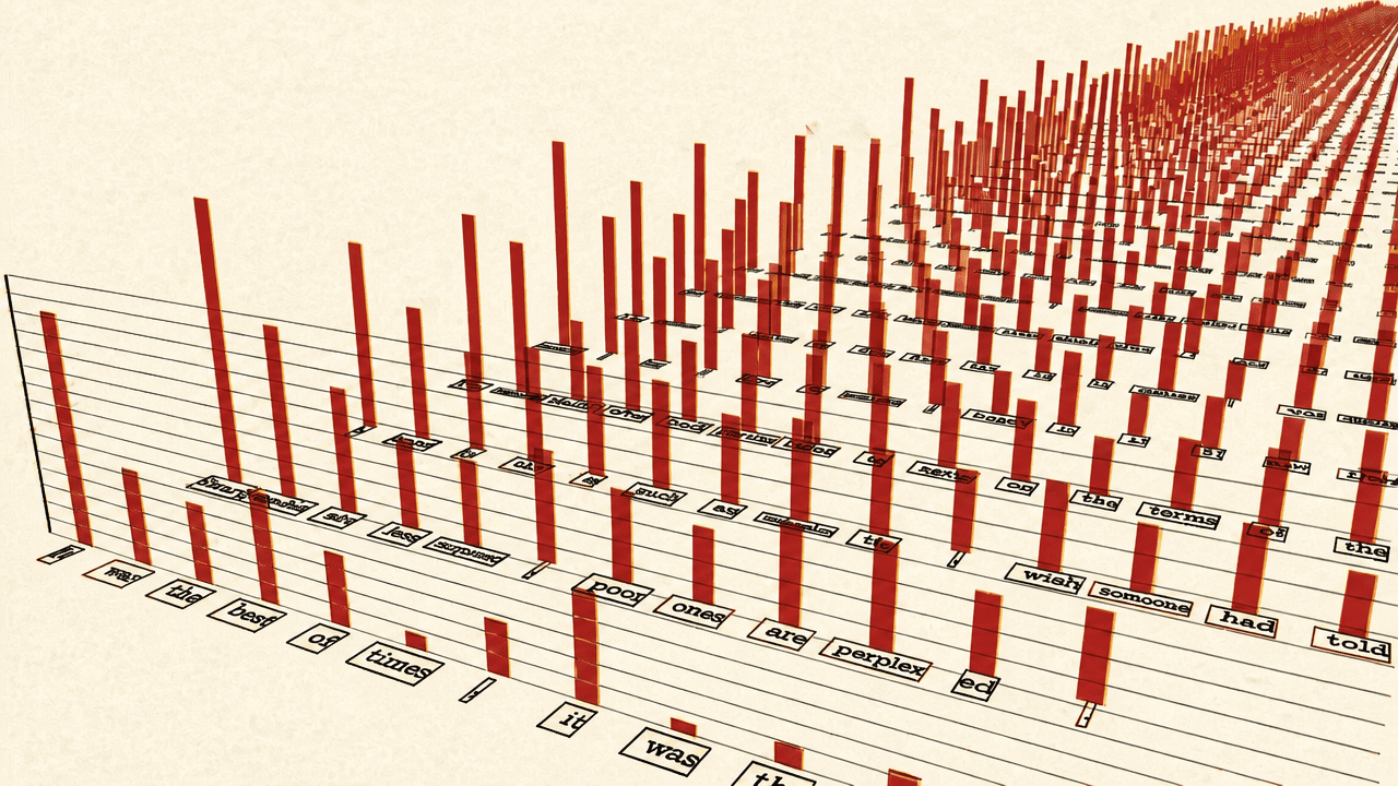
Cross-entropy is the cost of a mismatched probability model
A compression scheme is built around expectations. Symbols expected to occur often receive short codes; symbols expected to be rare can receive longer ones. Cross-entropy measures what happens when the expectations built into a code do not match the distribution that actually produces the data.
Grant Sanderson develops the idea with a robot receiving four instructions. Under the original distribution, “up” occurs half the time, “down” one quarter, and “left” and “right” one eighth each. An optimal binary code assigns one bit to up, two to down, and three to each of left and right. More generally, a symbol assigned probability receives a code length of approximately:


This is the information content of an event: the number of successive halvings needed to reach its probability. A 50% event contains one bit, a 25% event two bits, and a 12.5% event three. For a message, those quantities add: its optimal encoded length is approximately the sum of the information contents of its symbols.
Then the robot’s behavior changes without changing the code. Up and down each occur one eighth of the time, left one quarter, and right one half. The original encoder still gives up one bit, down two, and left and right three each.
| Instruction | Old probability and code | New probability | Cost under old code |
|---|---|---|---|
| Up | 1/2; 1 bit | 1/8 | 1/8 bit |
| Down | 1/4; 2 bits | 1/8 | 1/4 bit |
| Left | 1/8; 3 bits | 1/4 | 3/4 bit |
| Right | 1/8; 3 bits | 1/2 | 1 1/2 bits |
The resulting average cost is:
The expected code length is no longer the entropy of the data source, because the code was optimized for the wrong distribution. Let describe the probabilities that actually generate symbols and describe the probabilities assumed by the code. Cross-entropy is:
The asymmetry is the point. The values determine what happens often enough to matter in the average. The values determine the cost the coding system imposes. Cross-entropy asks a directional question: how well does a scheme optimized for perform on data drawn from ?
That directionality explains why a skewed code can fail badly when reality is not skewed. If assigns 90% probability to one of two events and 10% to the other, it spends roughly 0.15 bits on the common event and 3.32 bits on the rare one. When actual outcomes are 50/50, the average cost is about 1.74 bits per symbol. Reversing the distributions gives a different result: a code built for 50/50 assigns one bit to either event, so it costs one bit whether reality is even or 90/10.
The central property is that, with fixed, cross-entropy reaches its minimum when the assumed distribution exactly matches the real one. The minimum is the entropy of :
If you think of P as fixed and Q as the variable, it takes on its smallest possible value when Q is equal to P, and more specifically, that smallest value is the entropy of P.
Entropy is the irreducible average code length for a matched model. Cross-entropy is the average cost when the model and the source differ.
GZIP turned compression mismatch into a language map
The 2002 paper Language Trees and Zipping, by Dario Benedetto, Emanuele Caglioti, and Vittorio Loreto, reported that general-purpose file compression could cluster documents by language and recover a tree of their shared lineage without pre-built linguistic knowledge.
Its procedure begins with two documents, and . Take a small sample from , append it to , compress the result, and compare its size with compressing alone:
The increment asks how well the snippet from compresses after the compressor has been exposed mostly to the patterns in . If the texts share patterns, the added sample should cost less; if their patterns differ, it should cost more. The paper used this general idea to build a distance measure that, as presented here, grouped documents into recognizable language families.
The full measure was more complicated than the increment alone. It defined a document difference using the incremental compression costs of the same sample under each document:
But the essential question is the same one posed by cross-entropy: how does a coding scheme adapted to one context perform on data from another?
Sanderson is explicit that this is not literally cross-entropy. A document is a finite sample rather than an explicit probability distribution, and GZIP is far from an optimal compressor at the Shannon limit. Its underlying approach is comparatively direct: it finds repeated sequences and replaces later instances with pointers to earlier ones. The file-size increment is therefore a crude empirical estimate of a cross-entropy-like quantity, not a calculation of cross-entropy itself.
That limitation is part of what makes the example useful. A rough compressor was still sufficient, according to the paper’s reported result, to extract enough shared structure for language clustering; the same general trick can also be used for tasks such as authorship identification. Compression need not understand linguistic categories in advance to register that one body of text makes another more or less predictable.
Pre-training turns information into an objective
A language model maps a sequence of tokens—typically words or pieces of words—to a probability distribution over possible next tokens. Its training objective is evaluated over a large body of text, and gradient descent and backpropagation adjust the model’s many parameters to reduce that objective.
Grant Sanderson frames the loss as average information from the model’s perspective. At each position, the model assigns some probability to the token that actually appears next. That token contributes:
A high assigned probability produces little loss. A low one produces a steep penalty. The pre-training loss is the average of this quantity over the tokens in the training set. Base 2 expresses the result in bits; machine-learning practice generally uses natural logs, which differ only by a constant factor and are more convenient when taking derivatives.
The usual one-hot description is mathematically correct: treat the observed next token as a target distribution that puts all its probability mass on that token, and cross-entropy collapses to its negative log probability. But that shorthand does not explain why logarithms are the appropriate loss.
Consider many occurrences of the prefix “My name is.” Let be the frequency with which name follows that prefix in the data, and let be the model’s predicted probability for it. If the loss for one outcome is some generic function , then the average loss across such examples is:
Choosing produces cross-entropy:
The earlier minimum property now becomes an objective: this expected loss is minimized when the model’s distribution matches the distribution represented by the data.
Sanderson’s stronger claim is that the logarithm is effectively forced if that is the property one requires. Under the constraint that predicted probabilities sum to one, the constrained optimization implies that the derivative of the per-example loss must have the form:
Only a logarithm has a derivative proportional to . Negative-log loss is not simply one decreasing penalty among many. It is the choice that makes minimizing expected loss correspond to matching the relevant distribution.
There is an important qualification. A model should not literally reproduce the observed relative frequencies after every prefix: most prefixes have sparse evidence, often only one observed continuation, and literal reproduction would be overfitting. The inaccessible target is the underlying distribution from which the data was sampled. Training can only use the data available to nudge the model in that direction. Sanderson notes the striking consequence: models can produce reasonable continuations for text strings they have never seen, suggesting they learn something more abstract than a table of local observed frequencies.
Distillation replaces one hard target with a teacher's judgment
Distillation makes cross-entropy explicit rather than collapsing it to one observed token. A smaller model is trained to approximate a larger, presumably more capable model, with the aim of retaining useful performance in a system that is cheaper to run at inference time.
Grant Sanderson contrasts the target supplied by ordinary pre-training with the target supplied by a larger model. Pre-training gives full weight to one token: the continuation that appeared in the dataset. In distillation, the larger model supplies a full probability distribution across possible next tokens. The small model minimizes:
Here is the large model’s probability for token , and is the smaller model’s. A teacher distribution communicates not just which token happened to occur, but which alternatives it considers plausible and how heavily it weights them.
Sanderson compares the difference to learning chess by merely watching games versus having a stronger player explain the good moves available at each turn and their relative merits. In the “My name is” example, the student does not need thousands or millions of occurrences before its objective reflects a broad distribution of possible names. One teacher prediction can provide that distribution directly.
KL divergence is the coding waste a matched model avoids
KL divergence isolates the avoidable part of cross-entropy cost:
Grant Sanderson describes the first term as the cost of using when reality follows . The second is the entropy of , the cost of a code matched to that reality. Their difference is wasted bits per symbol.
In the shifted robot example, the old code costs 2.625 bits per instruction while an optimal code for the new distribution costs 1.75 bits. The difference is 0.875 wasted bits per instruction.
The same quantity can be written more compactly as:
KL divergence is zero when the distributions match and grows as they differ. It is not a true distance metric, however, because it is asymmetric: the cost of using in a world governed by need not equal the cost of using in a world governed by .
For distillation, KL divergence and cross-entropy differ only by the teacher distribution’s entropy:
With the teacher fixed, is constant with respect to the student model . Minimizing KL divergence therefore yields the same optimization of the student as minimizing cross-entropy. Sanderson poses that consequence as a final exercise: despite KL divergence sounding more naturally like a distance measure, substituting it for cross-entropy in this fixed-teacher setting does not change the student’s optimum.